This article introduces the main differences between various optimization algorithms and how to choose the best optimization method.
What is an Optimization Algorithm?
The function of an optimization algorithm is to minimize (or maximize) the loss function E(x) by improving the training method.
Some parameters inside the model are used to calculate the deviation between the true values Y and the predicted values in the test set, based on these parameters, the loss function E(x) is formed.
For example, weights (W) and biases (b) are such internal parameters, generally used to compute output values, playing a major role in training neural network models.
The internal parameters of the model play a very important role in effectively training the model and producing accurate results. This is why we should use various optimization strategies and algorithms to update and compute the network parameters that affect model training and output, bringing them closer to or achieving optimal values.
Optimization algorithms are divided into two main categories:
1. First-Order Optimization Algorithms
This type of algorithm uses the gradient values of each parameter to minimize or maximize the loss function E(x). The most commonly used first-order optimization algorithm is gradient descent.
Function gradient: A multivariable expression of the derivative dy/dx, used to represent the instantaneous rate of change of y with respect to x. Often, to calculate the derivative of a multivariable function, the gradient is used in place of the derivative, and partial derivatives are used to compute the gradient. A main difference between the gradient and the derivative is that the gradient of a function forms a vector field.
Therefore, for single-variable functions, derivatives are used for analysis; while gradients are produced based on multivariable functions. More theoretical details will not be elaborated here.
2. Second-Order Optimization Algorithms
Second-order optimization algorithms use second derivatives (also known as Hessian methods) to minimize or maximize loss functions. Due to the high computational cost of second derivatives, this method is not widely used.
Detailed Explanation of Various Neural Network Optimization Algorithms
Gradient Descent
Gradient descent is one of the most important techniques and foundations when training and optimizing intelligent systems. The function of gradient descent is:
By finding the minimum, controlling variance, updating model parameters, and ultimately making the model converge.
The formula for updating network parameters is: θ=θ−η×∇(θ).J(θ), where η is the learning rate, and ∇(θ).J(θ) is the gradient of the loss function J(θ).
This is the most commonly used optimization algorithm in neural networks.
Today, gradient descent is mainly used for weight updates in neural network models, that is, updating and adjusting the model parameters in one direction to minimize the loss function.
The backpropagation technique introduced in 2006 made it possible to train deep neural networks. Backpropagation first computes the product of input signals and their corresponding weights during forward propagation, then applies the activation function to the sum of these products. This way of converting input signals into output signals is an important means of modeling complex nonlinear functions and introduces nonlinear activation functions, allowing the model to learn almost any form of function mapping. Then, during the backpropagation process of the network, relevant errors are transmitted back, using gradient descent to update weight values by calculating the gradient of the error function E with respect to the weight parameter W, updating the weight parameters in the opposite direction of the loss function gradient.
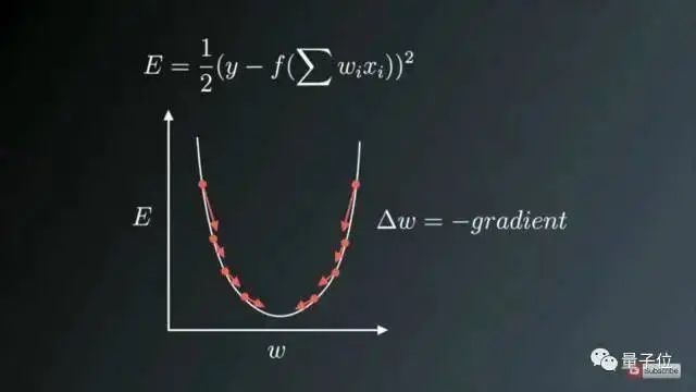
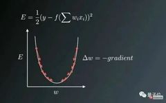
Figure 1: The direction of weight updates is opposite to the gradient direction
Figure 1 shows the weight update process against the direction of the gradient vector error, where the U-shaped curve represents the gradient. It should be noted that when the weight value W is too small or too large, there will be a significant error, necessitating the update and optimization of the weights to convert them into appropriate values, thus we attempt to find a local optimal value in the direction opposite to the gradient.
Variants of Gradient Descent
Traditional batch gradient descent calculates the gradient of the entire dataset but only performs one update, making it slow and difficult to control when dealing with large datasets, even leading to memory overflow.
The speed of weight updates is determined by the learning rate η, and it can converge to the global optimum on convex error surfaces, while it may tend toward local optimum on non-convex surfaces.
Using the standard form of batch gradient descent also has the problem of redundant weight updates when training on large datasets.
The aforementioned problems with standard gradient descent are solved in the stochastic gradient descent method.
1. Stochastic Gradient Descent (SGD)
Stochastic gradient descent (SGD) updates parameters for each training sample, performing one update each time, and executes faster.
θ=θ−η⋅∇(θ) × J(θ;x(i);y(i)), where x(i) and y(i) are the training samples.
Frequent updates result in high variance among parameters, causing the loss function to fluctuate with varying intensity. This is actually a good thing, as it helps us discover new and potentially better local minima, while standard gradient descent would only converge to a certain local optimum.
However, the issue with SGD is that due to the frequent updates and fluctuations, it will ultimately converge to a minimum and may exhibit overshooting due to frequent fluctuations.
It has been shown that when the learning rate η is gradually decreased, the convergence pattern of standard gradient descent is similar to that of SGD.
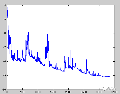
Figure 2: High variance in parameter updates for each training sample causes significant fluctuations in the loss function, thus we may not achieve the minimum of the loss function.
Another variant known as mini-batch gradient descent can address the problems of high variance parameter updates and unstable convergence.
2. Mini-Batch Gradient Descent
To avoid the issues present in SGD and standard gradient descent, an improved method is mini-batch gradient descent, where this method performs only one update for n training samples in each batch.
The advantages of using mini-batch gradient descent are:
1) It can reduce the fluctuations in parameter updates, ultimately achieving better and more stable convergence.
2) It can also utilize commonly used matrix optimization methods in the latest deep learning libraries, making the gradient computation for mini-batch data more efficient.
3) Generally, the range of mini-batch sample sizes is from 50 to 256, which can vary based on the actual problem.
4) When training neural networks, mini-batch gradient descent is usually chosen.
This method is sometimes referred to as SGD.
Challenges Faced When Using Gradient Descent and Its Variants
1. It is difficult to choose an appropriate learning rate. A learning rate that is too small can lead to slow convergence, while a learning rate that is too large may affect convergence, causing the loss function to fluctuate around the minimum, or even cause gradient divergence.
2. Moreover, the same learning rate does not apply to all parameter updates. If the training dataset is sparse and features have very different frequencies, they should not all be updated to the same extent, but a larger update rate should be used for infrequent features.
3. Another key challenge in neural networks when minimizing non-convex error functions is avoiding getting stuck in multiple other local minima. In fact, the problem does not stem from local minima but from saddle points, which are points that incline in one dimension and decline in another. These saddle points are often surrounded by planes with the same error value, making it difficult for the SGD algorithm to escape, as the gradient approaches zero in all dimensions.
Further Optimizing Gradient Descent
Now we will discuss various algorithms used for further optimizing gradient descent.
1. Momentum
The high variance oscillation in the SGD method makes it difficult for the network to converge stably, so researchers have proposed a technique called momentum, which optimizes training in relevant directions and weakens oscillation in irrelevant directions, to accelerate SGD training. In other words, this new method adds the component of the update vector from the previous step ‘γ’ to the current update vector.
V(t)=γV(t−1)+η∇(θ).J(θ)
Finally, the parameters are updated by θ=θ−V(t).
The momentum term γ is usually set to 0.9 or a similar value.
The momentum here is consistent with the momentum in classical physics, just like throwing a ball from a hill, collecting momentum during the fall, and the ball’s speed increases continuously.
In the parameter update process, the principle is similar:
1) It enables the network to converge better and more stably;
2) It reduces the oscillation process.
When the gradient points in the actual movement direction, the momentum term γ increases; when the gradient is opposite to the actual movement direction, γ decreases. This approach means that the momentum term only updates parameters for relevant samples, reducing unnecessary parameter updates, thus achieving faster and more stable convergence while reducing the oscillation process.
2. Nesterov Accelerated Gradient
A researcher named Yurii Nesterov pointed out a problem with the momentum method:
If a ball rolls down a slope blindly, it is very inappropriate. A smarter ball should pay attention to where it is going, so when it tilts back up the slope, the ball should slow down.
In fact, when the ball reaches the lowest point on the curve, the momentum is quite high. Due to the high momentum, it may completely miss the minimum, so the ball does not know when to slow down and continues to move upward.
Yurii Nesterov published a paper in 1983 addressing the momentum issue, hence we call this method Nesterov Accelerated Gradient.
In this method, he proposed to take a large leap based on previous momentum, then calculate the gradient for correction, thus achieving parameter updates. This pre-update method can prevent large oscillations and not miss the minimum, while being more sensitive to parameter updates.
Nesterov Accelerated Gradient (NAG) is a method that endows the momentum term with foresight, by using the momentum term γV(t−1) to change the parameters θ. By calculating θ−γV(t−1), we obtain an approximate value for the next position of the parameters, where the parameters are a rough concept. Thus, we do not calculate the gradient value of the current parameter θ but effectively foresee the future based on the approximate future position of relevant parameters:
V(t)=γV(t−1)+η∇(θ)J( θ−γV(t−1) ), then use θ=θ−V(t) to update the parameters.
Now, by making the network updates adapt to the slope of the error function, we can also adjust and update corresponding parameters based on the importance of each parameter, to perform larger or smaller updates.
3. Adagrad Method
The Adagrad method adjusts the appropriate learning rate η based on the parameters, making large updates for sparse parameters and small updates for frequent parameters. Therefore, the Adagrad method is very suitable for handling sparse data.
In each time step, the Adagrad method sets different learning rates for different parameters θ based on past gradients calculated for each parameter.
Previously, each parameter θ(i) used the same learning rate, updating all parameters θ each time. In each time step t, the Adagrad method selects different learning rates for each parameter θ, updates the corresponding parameters, and then vectorizes. For simplicity, we denote the loss function gradient for parameter θ(i) at time t as g(t,i).
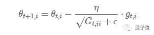
Figure 3: Parameter update formula
The Adagrad method modifies the corresponding learning rate η for each parameter θ(i) based on the previously calculated parameter gradients at each time step.
The main advantage of the Adagrad method is that it does not require manual adjustment of the learning rate. Most parameters use the default value of 0.01 and remain unchanged.
The main disadvantage of the Adagrad method is that the learning rate η always decreases and decays.
Since each additional term is positive, the accumulated sum of multiple squared gradient values in the denominator keeps growing during training. This, in turn, leads to the learning rate decreasing to very small magnitudes, causing the model to completely stop learning and stop acquiring new additional knowledge.
As the learning speed decreases, the model’s learning ability rapidly declines, and the convergence speed becomes very slow, requiring a long time for training and learning, i.e., the learning speed decreases.
Another algorithm called Adadelta improves this problem of continuously decaying learning rates.
4. Adadelta Method
This is an extension of the AdaGrad method that seeks to resolve the issue of learning rate decay. Adadelta does not accumulate all previous squared gradients but limits the window of accumulated previous gradients to a fixed size w.
Unlike previously ineffective storage of w previous squared gradients, the sum of gradients is recursively defined as the exponentially decaying average of all previous squared gradients. Similar to the momentum term, the sliding average Eg² at time t depends only on the previous average and the current gradient value.
Eg²=γ.Eg²+(1−γ).g²(t), where γ is set to a value close to the momentum term, around 0.9.
Δθ(t)=−η⋅g(t,i).
θ(t+1)=θ(t)+Δθ(t)
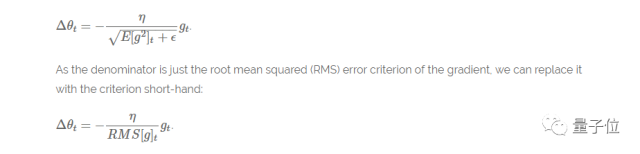
Figure 4: Final formula for parameter updates
Another advantage of the Adadelta method is that it no longer requires setting a default learning rate.
Improvements Made So Far
1) Different learning rates calculated for each parameter;
2) Also calculated the momentum term;
3) Prevented issues such as learning rate decay or vanishing gradients.
What Further Improvements Can Be Made?
In previous methods, learning rates corresponding to each parameter were calculated, but why not calculate the corresponding momentum changes for each parameter and store them independently? This is the improvement point proposed by the Adam algorithm.
Adam Algorithm
The Adam algorithm stands for Adaptive Moment Estimation, which can calculate adaptive learning rates for each parameter. This method not only stores the exponentially decaying average of previous squared gradients from AdaDelta but also maintains the exponentially decaying average of previous gradients M(t), similar to momentum:
M(t) is the first moment average of the gradient, and V(t) is the second moment non-central variance of the gradient.
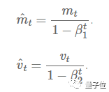
Figure 5: The two formulas represent the first moment average and the second moment variance of the gradient
Thus, the final formula for parameter updates is:
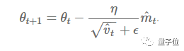
Figure 6: Final formula for parameter updates
Where β1 is set to 0.9, β2 is set to 0.9999, and ϵ is set to 10-8.
In practical applications, the Adam method performs well. Compared to other adaptive learning rate algorithms, it converges faster, is more effective in learning, and can correct issues present in other optimization techniques, such as vanishing learning rates, slow convergence, or high variance in parameter updates leading to large fluctuations in the loss function.
Visualizing Optimization Algorithms
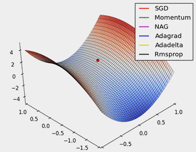
Figure 7: SGD optimization on saddle points
From the above animation, it can be seen that adaptive algorithms can converge quickly and find the correct target direction in parameter updates; while standard SGD, NAG, and momentum methods converge slowly and find it difficult to determine the correct direction.
Conclusion
Which optimizer should we use?
When building neural network models, it is crucial to choose the best optimizer to achieve fast convergence and correct learning while adjusting internal parameters to minimize the loss function to the greatest extent.
Adam performs well in practical applications, surpassing other adaptive techniques.
If the input dataset is relatively sparse, methods like SGD, NAG, and momentum may not perform well. Therefore, for sparse datasets, some form of adaptive learning rate method should be used, with the additional benefit of not requiring manual adjustment of the learning rate, as default parameters may yield optimal values.
If you want to make the training of deep network models converge quickly or if the constructed neural network is complex, you should use Adam or other adaptive learning rate methods, as these methods tend to be more effective in practice.
I hope that through this article, you can gain a good understanding of the differences in characteristics among various optimization algorithms.
Related Links:
Second-Order Optimization Algorithms: https://web.stanford.edu/class/msande311/lecture13.pdf
Nesterov Accelerated Gradient: http://cs231n.github.io/neural-networks-3/