Table of Contents
1. Principles of KNN Algorithm
2. Three Elements of KNN Algorithm
3. Brute Force Implementation of KNN Algorithm
4. KD-Tree Implementation of KNN Algorithm
5. Imbalance in Training Samples for KNN Algorithm
6. Advantages and Disadvantages of the Algorithm
1. Principles of KNN Algorithm
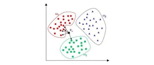
The KNN algorithm selects the k nearest training samples to the input sample in the feature space and provides an output result based on a certain decision rule.
Decision Rules:
For classification tasks: The output result is the class that occurs most frequently among the k training samples.
For regression tasks: The output result is the average of the values of the k training samples.
In the classification task shown in the figure below, the output result is class w1.
2. Three Elements of KNN Algorithm
The choice of K value, distance metric, and classification decision rule are the three basic elements of the K-Nearest Neighbors algorithm. Once these three elements are determined, the Y value for any new input instance is also determined. This section introduces the meaning of these three elements.
1. Classification Decision Rule
The KNN algorithm generally uses a majority voting method, where the class of the input instance is determined by the majority class of its K nearest neighbors. This idea is also a result of empirical risk minimization.
The training samples are (xi, yi). When the input instance is x, labeled as c, is the k nearest training sample set for input instance x.
We define training error rate as the proportion of the K nearest training samples’ labels that are inconsistent with the input label, represented as:
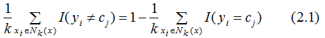
Therefore, to minimize the error rate, i.e., to minimize empirical risk, we need to maximize the right-hand side of equation (2.1),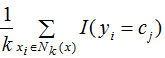 which means that the label values of the K nearest neighbors should be as consistent as possible with the input labels. Therefore, the majority voting rule is equivalent to minimizing empirical risk.
2. Choice of K Value:
When K is small, the model complexity is high, training error will decrease, but generalization ability weakens; when K is large, model complexity is low, training error increases, but generalization ability improves to some extent.
The complexity of the KNN model can be understood through its tolerance to noise. If the model is very sensitive to noise, its complexity is high; conversely, if the model is less sensitive to noise, its complexity is low. To better understand the meaning of model complexity, we take an extreme case and analyze the model complexities for K=1 and K=”number of samples”.
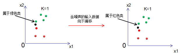
From the above figure, we can see that when K=1, the results output by the model are greatly affected by noise.
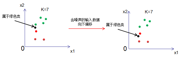
From the above figure, we can see that when the number of samples is 7, when K=7, regardless of how much noise is present in the input data, the output result is always the green class. The model is extremely insensitive to noise, but the model is too simple and contains too little information, which is also undesirable.
From the above two extreme K selection results, we can conclude that the choice of K should be moderate, generally less than 20, and it is recommended to use cross-validation to select an appropriate K value.
3. Distance Metric
The KNN algorithm uses distance to measure the similarity between two samples. Common distance metrics include:
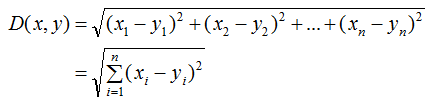
(1) Euclidean Distance
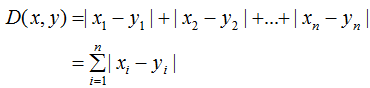
(2) Manhattan Distance
(3) Minkowski Distance
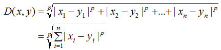
It can be seen that the Euclidean distance is a special case of Minkowski distance when p=2, while the Manhattan distance is a special case when p=1.
3. Brute Force Implementation of KNN Algorithm
Brute-force search is a linear scan of the input instance against each training instance to find the distances and select the top k nearest neighbors for majority voting. The algorithm is simple, but when the training set or feature dimensions are large, the computation is very time-consuming, making this brute-force implementation impractical.
4. KD-Tree Implementation of KNN Algorithm
A KD-tree is a tree data structure that stores instance points in k-dimensional space for fast retrieval. Constructing a KD-tree involves repeatedly partitioning the k-dimensional space with hyperplanes perpendicular to the axes, creating a series of k-dimensional hyper-rectangles. The KD-tree eliminates the need to search most of the data, significantly reducing the computational load.
The KNN algorithm implementation using KD-tree includes three parts: constructing the KD-tree, searching the KD-tree, and classifying using the KD-tree.
1. Constructing the KD-tree
The KD-tree is essentially a binary tree, and its partitioning idea is consistent with that of a CART tree, i.e., splitting the feature that reduces sample complexity the most. The KD-tree prioritizes features with higher variance for splitting, where the split point is the median of all instances in that feature. This splitting process is repeated until no samples are left to split, at which point the samples become leaf nodes.
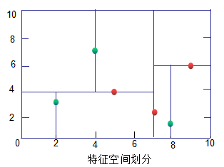
[Example] Given a dataset in a two-dimensional space:

Steps to construct the KD-tree:
(1) The variances of the dataset in the dimensions and
and are 6.9 and 5.3, respectively, so we first split along
 dimension.
(2) The median of the dataset in dimension is 7. The space is divided into two rectangles at the plane
 =7.
=7.
(3) The samples in the left and right rectangles are split based on the median in dimension.
(4) Repeat steps (2) and (3) until no samples are left, at which point that node becomes a leaf node.
As shown in the figure below, green indicates leaf nodes, while red indicates nodes and the root node.
2. KD-Tree Search
(1) The search path goes from the root node to the leaf node, finding the leaf node that contains the target point in the KD-tree.
(2) The search path goes from the leaf node back to the root node, finding the sample instance that is closest to the target point. The process is not repeated here; for specific methods, please refer to Dr. Li Hang’s “Statistical Learning Methods”.
3. KD-Tree Prediction
Each search finds the sample node closest to the input sample, then ignores that node and repeats the same steps K times to find the K nearest samples to the input sample, using majority voting to determine the output result.
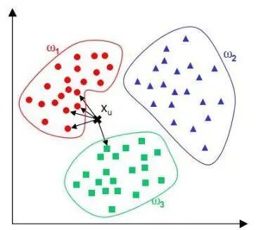
5. Imbalance in Training Samples for KNN Algorithm
If positive and negative samples are in an imbalanced state, the KNN algorithm using voting decisions will determine the class of the input sample:
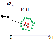
The result shows that the input sample is of the green class. The reason is that the number of red classes is far less than that of green samples, leading to classification errors.
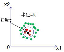
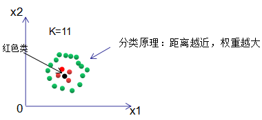
(1) If the classification decision chooses a limited radius nearest neighbor method, i.e., selecting the class that appears most frequently within a circle of radius R centered at the input sample, as shown in the figure, the classification result for the black sample is correct.
(2) The voting method assumes equal weight for each sample. We assume that the weight is inversely proportional to the distance, meaning that the farther away a sample is, the less impact it has on the result, thus its weight is smaller; conversely, the closer the sample is, the greater its weight. The classification of the input sample is based on this weight. This idea is similar to the AdaBoost algorithm, where weak classifiers with good classification performance are given higher weights.
Classification Process:
(1) Select the K training samples Xi (i = 1,2,…,K) that are closest to the input sample X0, where d(X0,Xi) represents the distance between the input sample and the training sample.
(2) Convert the distances into weights Wi, which represent the weights of the input sample X0 relative to the training samples Xi, based on the property of distance being inversely proportional to the sample.
(3) We accumulate the weights of each class of samples and consider the proportion of that weight to the total weight as the probability of that class. The class with the highest probability is the classification result for the input sample.
Assuming the target is a binary classification {C1, C2}, the expression is:
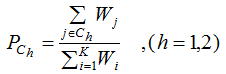
If , then the classification result is class C1, otherwise class C2.
Regression Process:
(1) and (2) steps are the same as in the classification process, while step (3) uses the following expression to obtain the regression value:
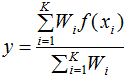
where y is the output result, and f(xi) is the value of the nearest neighbor samples. If the weights are the same, the output result will be the average of the K training samples.
Using the weight concept to reclassify the above example, we find that the input sample belongs to the red class.
6. Advantages and Disadvantages of the KNN Algorithm
Advantages:
1) The algorithm is simple, theoretically mature, and can be used for classification and regression.
2) It is insensitive to outliers.
3) It can be used for non-linear classification.
4) It is more suitable for large training datasets, while small datasets are prone to misclassification.
5) The principle of the KNN algorithm is to determine the output class based on the K samples in the neighborhood, making KNN more suitable than other methods for sample sets with significant overlap between different classes.
Disadvantages:
1) High time complexity and space complexity.
2) Imbalanced training samples lead to low prediction accuracy for rare classes.
3) Compared to decision tree models, KNN models have weaker interpretability.
References:
https://www.cnblogs.com/pinard/p/6061661.html
Recommended Reading
Summary of XGBoost Algorithm Principles
Discussion on Logistic Function and Softmax Function
Summary of Random Forest Algorithm

-END-