The k-means algorithm is one of the most commonly used methods for unsupervised clustering due to its simplicity and good applicability to large sample data. This article provides a detailed summary of the principles of the k-means clustering algorithm.
Table of Contents
1. Principles of k-means Clustering Algorithm
2. Steps of k-means Clustering Algorithm
3. k-means++ Clustering Optimization Algorithm
4. Mini-batch Processing of k-means Clustering Algorithm
5. Selecting the Value of k
6. Scenarios Where k-means Clustering Algorithm Is Not Applicable
7. Differences Between k-means and KNN
8. Conclusion
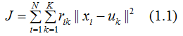
An article on the performance measurement of clustering algorithms mentions that if the similarity within clusters is high and the similarity between clusters is low, then the performance of the clustering algorithm is good. Based on this, we define the objective function of the k-means clustering algorithm:
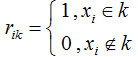
Where  indicates that when a sample is assigned to cluster k, the value is 1, otherwise it is 0.
 represents the mean vector of cluster k.
The objective function (1.1) characterizes the compactness of samples within the cluster around the mean vector to some extent; the smaller the value of J, the higher the similarity of samples within the cluster. Minimizing the objective function is an NP-hard problem; the k-means clustering uses the EM algorithm concept to achieve model optimization.
1) Initialize the mean vectors of k clusters, i.e.,  is a constant, and find the minimum of
  . It is easy to see that when data points are assigned to the nearest cluster, the objective function J reaches its minimum.
2) Given  , find the corresponding
  that minimizes J. Set the partial derivative of the objective function J with respect to
  equal to 0:
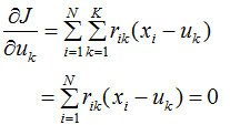
We obtain:
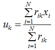
 means that the cluster center equals the mean of the samples belonging to that cluster.
This section explains the parameter update process of the k-means clustering algorithm using the EM algorithm concept, and we believe that everyone has a clearer understanding of the k-means clustering algorithm.
The steps of the k-means clustering algorithm essentially represent the model optimization process of the EM algorithm, and the specific steps are as follows:
1) Randomly select k samples as the initial mean vectors of the clusters;
2) Assign each sample in the dataset to the nearest cluster;
3) Update the mean vector of the clusters based on the samples assigned to each cluster;
4) Repeat steps (2) and (3) until the set number of iterations is reached or the mean vectors of the clusters no longer change, then the model is constructed, and the clustering results are output.
If given enough iterations, the k-means algorithm can converge, but it may converge at a local minimum. The reason for k-means converging to a local extreme is likely due to the close distances of the initialized cluster centers, which also prolongs the convergence time. To avoid this situation, run the k-means clustering algorithm multiple times, initializing different cluster centers each time.
Another solution to the local extreme convergence of k-means is the k++ clustering algorithm, which initializes the cluster centers by keeping them apart from each other.
Specific algorithm steps:
1) Randomly select a sample data point as the first cluster center ;
;
2) Calculate the minimum distance from each sample to the cluster center
 ;
;

3) Choose the sample point with the maximum distance as the cluster center;
4) Repeat steps (2) and (3) until reaching the number of clusters k;
5) Use these k cluster centers as the initialized cluster centers to run the k-means algorithm;
The time complexity of the k-means clustering algorithm increases with the number of samples. When the sample size reaches tens of thousands, the k-means clustering algorithm can be very time-consuming. Therefore, a suitable mini-batch sample dataset can be obtained through random sampling without replacement. The sklearn.cluster package provides the corresponding implementation method MiniBatchKMeans.
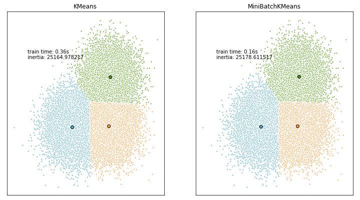
The mini-batch processing of the k-means clustering algorithm reduces convergence time while producing similar algorithm results. The following results use inertia to evaluate the results of k-means and MiniBatchKMeans.
import time

import numpy as np
import matplotlib.pyplot as plt

from sklearn.cluster import MiniBatchKMeans, KMeans
from sklearn.metrics.pairwise import pairwise_distances_argmin
from sklearn.datasets.samples_generator import make_blobs

# Generate sample data
np.random.seed(0)
# minibatch randomly sample 100 examples for training
batch_size = 100
centers = [[1, 1], [-1, -1], [1, -1]]
n_clusters = len(centers)
# Generate 30000 sample data for 3 clusters
X, labels_true = make_blobs(n_samples=30000, centers=centers, cluster_std=0.7)

# k-means++ algorithm
k_means = KMeans(init='k-means++', n_clusters=3, n_init=10)
t0 = time.time()
k_means.fit(X)
t_batch = time.time() - t0


# MiniBatchKMeans algorithm
mbk = MiniBatchKMeans(init='k-means++', n_clusters=3, batch_size=batch_size,
                      n_init=10, max_no_improvement=10, verbose=0)
t0 = time.time()
mbk.fit(X)
t_mini_batch = time.time() - t0

# Print k-means++ runtime and performance metrics
print("k-means++_runtime= ",t_batch)
print("k_means++_metics= ",k_means.inertia_)
# Print minibatch_k_means++ runtime and performance metrics
print("MiniBatch_k_means++_runtime= ",t_mini_batch)
print("k_means_metics= ",mbk.inertia_)

#>
k-means++_runtime=  0.36002039909362793
k_means++_metics=  25164.97821695812
MiniBatch_k_means++_runtime=  0.15800929069519043
k_means_metics=  25178.611517320118
The graphical results indicate:
We use the Calinski-Harabasz score as a standard to evaluate clustering performance. The higher the score, the better the clustering performance. The meaning of Calinski-Harabasz can be found in this article.
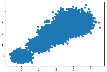
First, we construct two-dimensional sample data with four different standard deviations:
from sklearn import metrics
# Define four cluster centers
centers1 = [[0,0],[1, 1],[1.9, 2],[3, 3]]
# Define the standard deviation for each cluster
std1 = [0.19,0.2,0.3,0.4]
# Algorithm reproducibility
seed1 =45
# Generate 30000 sample data for 4 clusters
X, labels_true = make_blobs(n_samples=30000, centers=centers1, cluster_std=std1,random_state=seed1)
plt.scatter(X[:,0],X[:,1],marker='o')
plt.show()
The scatter plot of the data is as follows:
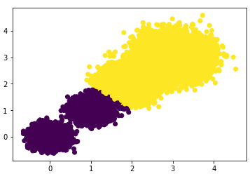
First, select the number of clusters as 2, i.e., K=2, and check the clustering effect and Calinski-Harabasz score.
# If we choose k=2
k_means = KMeans(init='k-means++', n_clusters=2, n_init=10,random_state=10)
y_pred = k_means.fit_predict(X)
plt.scatter(X[:, 0], X[:, 1], c=y_pred)
plt.show()
scores2 = metrics.calinski_harabaz_score(X,y_pred)
print("the Calinski-Harabasz scores(k=2) is: ",scores2)
Scatter plot effect:
Calinski-Harabasz score:
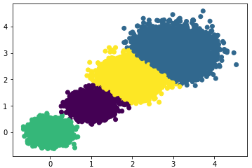
#> the Calinski-Harabasz scores(k=2) is: 85059.39875951338Select the number of clusters as 3, i.e., K=3, and check the clustering effect and Calinski-Harabasz score.
Scatter plot effect:
Calinski-Harabasz score:
#> the Calinski-Harabasz scores(k=3) is: 92778.08155077342
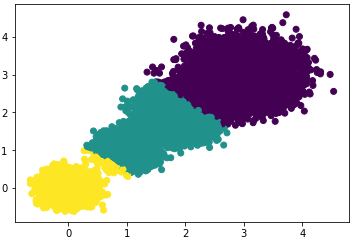
Select the number of clusters as 4, i.e., K=4, and check the clustering effect and Calinski-Harabasz score.
Scatter plot effect:
Calinski-Harabasz score:
#> the Calinski-Harabasz scores(k=4) is: 158961.98176157777From the results, it can be seen that the highest Calinski-Harabasz score is when k=4, so we choose the number of clusters as 4.
The k-means algorithm assumes that the data is isotropic, meaning that the covariance of different clusters is equal. In simple terms, the probability of sample data falling in all directions is equal.
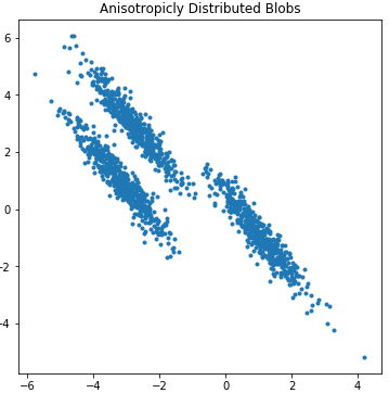
1) If the sample data is anisotropic, the k-means algorithm performs poorly.
Generate a set of anisotropic sample data:
import numpy as np
import matplotlib.pyplot as plt

from sklearn.cluster import KMeans
from sklearn.datasets import make_blobs

plt.figure(figsize=(6, 6))

n_samples = 1500
random_state = 170
X, y = make_blobs(n_samples=n_samples, random_state=random_state)

# Generate anisotropic data
transformation = [[0.60834549, -0.63667341], [-0.40887718, 0.85253229]]
X_aniso = np.dot(X, transformation)

plt.scatter(X_aniso[:, 0], X_aniso[:, 1], marker='.')
plt.title("Anisotropically Distributed Blobs")

plt.show()
Scatter plot effect of generated sample data:
Based on the scatter plot distribution, we train the sample data using k=3:
# Train data with k=3, output scatter effect diagram
y_pred = KMeans(n_clusters=3, random_state=random_state).fit_predict(X_aniso)
plt.scatter(X_aniso[:, 0], X_aniso[:, 1], marker='.',c=y_pred)
plt.title("clustering scatter distributed k=3")
plt.show()
Clustering effect diagram:
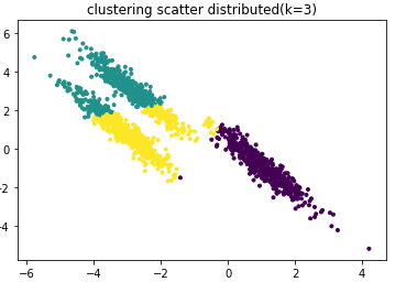
From the above figure, it can be seen that the clustering effect is poor.
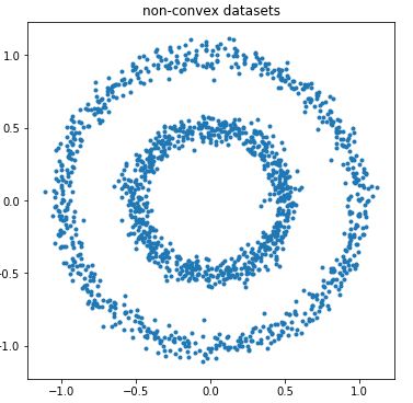
2) When the sample dataset is non-convex, the k-means clustering effect is poor:
First, generate a non-convex dataset:
# Non-convex dataset
plt.figure(figsize=[6,6])
from sklearn import cluster,datasets
n_samples = 1500
noisy_circles = datasets.make_circles(n_samples=n_samples, factor=.5, noise=.05)
plt.scatter(noisy_circles[0][:,0],noisy_circles[0][:,1],marker='.')
plt.title("non-convex datasets")
plt.show()
Scatter plot effect:
Based on the scatter plot distribution, we train the sample data using k=2:
# Train data with k=2
y_pred = KMeans(n_clusters=2, random_state=random_state).fit_predict(noisy_circles[0])
plt.scatter(noisy_circles[0][:, 0], noisy_circles[0][:, 1], marker='.',c=y_pred)
plt.title("non-convex k-means clustering")
plt.show()
Scatter plot clustering effect:
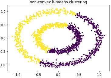
From the above figure, it can be seen that the clustering effect is poor.
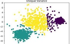
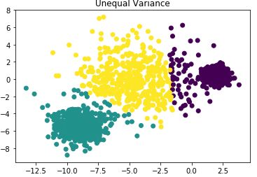
3) If the standard deviations of each cluster are not equal, the k-means clustering effect is poor.
# Construct data for each cluster with different variances, standard deviations are 1.0, 2.5, 0.5
X_varied, y_varied = make_blobs(n_samples=n_samples,
                                cluster_std=[1.0, 2.5, 0.5],
                                random_state=random_state)
y_pred = KMeans(n_clusters=3, random_state=random_state).fit_predict(X_varied)

plt.scatter(X_varied[:, 0], X_varied[:, 1], c=y_pred)
plt.title("Unequal Variance")
plt.show()
From the figure below, it can be seen that the clustering effect is poor:
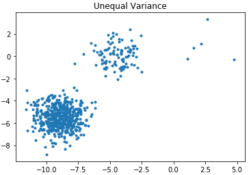
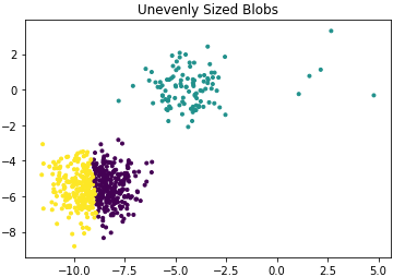
4) If the number of samples in each cluster differs significantly, the clustering performance is poor.
Generate three clusters with sample sizes of 500, 10, and 10:
n_samples = 1500
random_state = 170
# Generate three clusters, each with 500 samples
X, y = make_blobs(n_samples=n_samples, random_state=random_state)
# The sample sizes of the three clusters are 500, 100, and 10, check the clustering effect
X_filtered = np.vstack((X[y == 0][:500], X[y == 1][:100], X[y == 2][:5]))
plt.scatter(X_filtered[:, 0], X_filtered[:, 1], marker='.')
plt.title("Unequal Variance")
plt.show()
Scatter plot distribution:
Use k-means to cluster:
y_pred = KMeans(n_clusters=3,
                random_state=random_state).fit_predict(X_filtered)
plt.scatter(X_filtered[:, 0], X_filtered[:, 1], c=y_pred,marker='.')
plt.title("Unevenly Sized Blobs")

plt.show()
Effect diagram as follows:
5) If the data dimensions are very high, the runtime will be long; consider first using PCA for dimensionality reduction.
# Generate 100-dimensional samples with 15000 samples
n_samples = 15000
random_state = 170
plt.figure(figsize=[10,6])
t0=time.time()
# Generate three clusters, each with 500 samples
X, y = make_blobs(n_samples=n_samples, n_features=100,random_state=random_state)
y_pred = KMeans(n_clusters=3,
                random_state=random_state).fit_predict(X)
t1 =time.time()-t0
scores1 = metrics.calinski_harabaz_score(X,y)
print("no feature dimonsion reduction scores = ",scores1)
print("no feature dimonsion reduction runtime = ",t1)
Output clustering effect and runtime:
no feature dimonsion reduction scores =  164709.2183791984
no feature dimonsion reduction runtime =  0.5700197219848633
Data is first reduced by PCA and then clustered using k-means,
# Data first PCA dimensionality reduction, then k-means clustering
from sklearn.decomposition import PCA
pca = PCA(n_components=0.8)
s=pca.fit_transform(X)
t0=time.time()
y_pred = KMeans(n_clusters=3,
                random_state=random_state).fit_predict(s)
t1 = time.time()-t0
print("feature dimonsion reduction scores = ",scores1)
print("feature dimonsion reduction runtime = ",t1)
Output clustering effect and runtime:
feature dimonsion reduction scores =  164709.2183791984
feature dimonsion reduction runtime =  0.0630037784576416
From the comparative results, it can be seen that while the clustering effects are similar, the runtime has been greatly reduced.
k-means is the simplest unsupervised classification algorithm, while KNN is the simplest supervised classification algorithm. Beginners may feel a sense of familiarity when learning unsupervised chapters after completing the supervised learning chapter, possibly because both use distance as a measure of similarity between samples. Below are several differences:
1) KNN is a supervised learning method, while k-means is an unsupervised learning method, hence KNN requires labeled classes for samples, while k-means does not;
2) KNN does not require training; it simply finds the k nearest samples to the test sample and gives classification results based on the classes of those k samples; k-means requires training to obtain the mean vectors (centroids) of each cluster, and classifies test data based on the centroids;
The k-means algorithm is simple and performs well with large sample data, which has led to its wide application. This article also lists several scenarios where k-means is not applicable. Other clustering algorithms may effectively address the scenarios that k-means cannot solve. Different clustering algorithms have their own advantages and disadvantages. Subsequent articles will continue to introduce clustering algorithms, and I hope this summary article on k-means can be helpful to you.
References
https://scikit-learn.org/stable/modules/clustering.html#clustering
https://www.cnblogs.com/pinard/p/6169370.html
Recommended Reading
Clustering | A Detailed Summary of Performance Metrics and Similarity Methods