
Statistical Classification Methods: (1) Based on KNN (K-Nearest Neighbors): Use similarity to find the k nearest training samples, then score and rank them by score. (2) Based on Naive Bayes Algorithm: Calculate probabilities to build classification models.
Guidance:
A doctor diagnosing a patient is a typical classification process. No doctor can directly see a patient’s condition; they can only infer the condition by observing the symptoms exhibited by the patient and various test data. In this case, the doctor acts as a classifier, and the accuracy of the diagnosis is closely related to their educational background (constructive method), whether the patient’s symptoms are prominent (characteristics of the data to be classified), and the doctor’s experience (number of training samples).
1.1.1 Nearest Neighbor Algorithm Definition: Calculate the distance between the unknown sample and all training samples, and use the category of the nearest neighbor as the sole basis for deciding the category of the unknown sample. Shortcoming: Too sensitive to noisy data. Measure: Include multiple nearest samples around the decision sample to expand the sample size involved in the decision, avoiding individual data from directly determining the decision outcome. 1.1.2 K-Nearest Neighbors (KNN) Basic Idea: Select K samples within a certain range of the unknown sample; the type that appears most frequently among these K samples determines the category of the unknown sample. Example: If K=3, the three nearest neighbors of the green dot are 2 red triangles and 1 blue square; the minority belongs to the majority, and based on statistical methods, the green point is classified as belonging to the red triangle type. If K=5, the five nearest neighbors of the green dot are 2 red triangles and 3 blue squares; again, the minority belongs to the majority, and based on statistical methods, the green point is classified as belonging to the blue square type.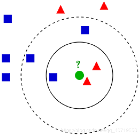 Algorithm Execution Steps: (1) Input the test set. (2) Set parameter k. (3) Traverse the test set; for each sample in the test set, calculate the distance from that sample to each sample in the training set; extract the k samples with the smallest distances from the training set to that sample; count the category labels of these samples; the category label that appears most frequently is the category label of that sample in the test set. (4) After traversal, output the categories of the test set.
1.1.3 Knowledge Supplement Distance metrics represent the degree of similarity between two samples. Commonly used distance metrics: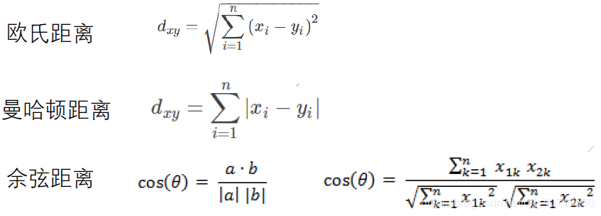
2.1 Bayes Formula Understanding of Bayes Formula https://www.zhihu.com/question/19725590/answer/241988854 (How to explain Bayes’ theorem in non-mathematical language?) 2.2 Naive Bayes Classifier 2.2.1 Basic Idea For a given item to be classified, calculate the probability of each category occurring given that item; the category with the highest probability is considered the category to which the item belongs.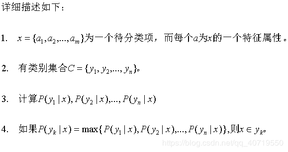 2.2.2 Naive Bayes “Formula”
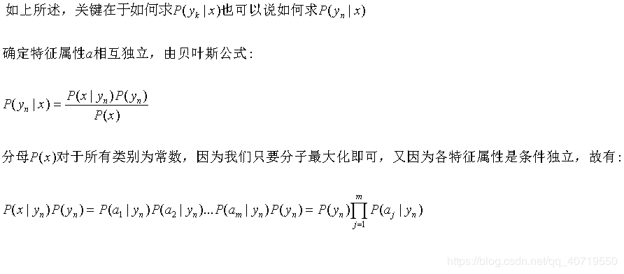
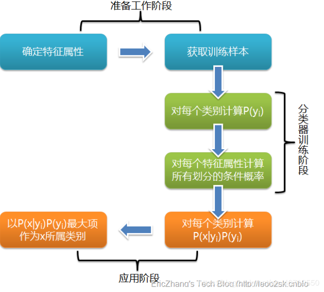 2.2.3 Naive Bayes Classifier
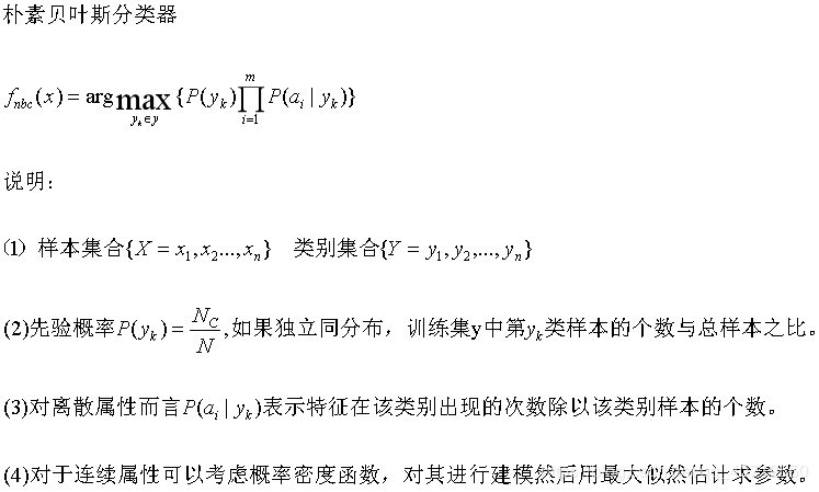
Detection Methods:
(1) Selection and extraction of defect image features. (2) Calculate the difference in grayscale between the defect image and the standard image. (3) Compare the difference with a set threshold to determine if a defect exists.
3.1 Defect Image Difference Method 3.1.1 Basic Principle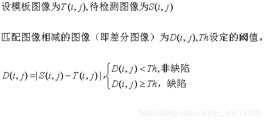 3.1.2 Basic Process (1) Set the effective detection area (2) Image registration and cropping (3) Set the difference threshold (4) Determine the defect location 3.2 Selection and extraction of defect image features See: https://zhuanlan.zhihu.com/p/43488853 3.2.1 Feature extraction methods (1) Grayscale features (2) Grayscale difference features (3) Histogram features (4) Transformation coefficient features (5) Line and corner features (6) Grayscale edge features (7) Texture features 3.2.2 Feature selection (Dimensionality reduction) Reason for dimensionality reduction: In machine learning, if the feature values (i.e., dimensions) are too many, it can lead to the curse of dimensionality. The most direct consequence of the curse of dimensionality is overfitting, which leads to classification errors. Therefore, we need to perform dimensionality reduction on the proposed features. Basic Principle: Feature selection transforms the original space to regenerate a feature space with smaller dimensions and more independent dimensions. Problems faced in dimensionality reduction: (1) Should the reduced data contain more information? (2) How much information will be lost after dimensionality reduction? (3) What impact will dimensionality reduction have on classification recognition? Benefits of data dimensionality reduction: (1) Data compression, reducing the storage space required and the computation time needed. (2) Eliminate redundancy between data to simplify data and improve computational efficiency. (3) Remove noise to enhance model performance. (4) Improve data comprehensibility and increase the accuracy of learning algorithms. (5) Reduce data dimensions to 2 or 3 for visualization. Common methods: Principal Component Analysis, Random Mapping, Non-negative Matrix Factorization. 3.2.3 Overview of Principal Component Analysis (PCA): The goal of this method is to find the most significant elements and structures in the data, remove noise redundancy, reduce the original complex data dimensions, and reveal the simple structures hidden behind complex data. PCA attempts to best simplify this multivariate data table while ensuring minimal loss of data information. These comprehensive indicators are called principal components, which means reducing the dimensionality of high-dimensional variable space. Clearly, it is much easier for a recognition system to operate in a low-dimensional space than in a high-dimensional space. From a linear algebra perspective, the goal of PCA is to find a new orthogonal basis to re-describe the data space, and this dimension is the principal component. 3.3 Grayscale Morphological Defect Detection 3.3.1 Overview The basic operations of grayscale mathematical morphology include dilation, erosion, opening, and closing, where the combination of dilation and erosion can form opening and closing, and the use of opening and closing can form morphological filters. In the morphological analysis of grayscale images, the structural elements can be any three-dimensional structure, commonly used shapes include cones, cylinders, hemispheres, or parabolas. The template size is always odd, so the center of the template corresponds exactly to a pixel. 3.3.2 Impact of Morphological Operations on Images (1) The result of dilating a grayscale image is that the brighter parts compared to the background expand, while the darker parts shrink. (2) The result of eroding a grayscale image is that the darker parts expand, while the brighter parts shrink. (3) Opening an image can eliminate isolated points or spikes that are too bright in the image. (4) Closing an image can remove structures that are darker than the background and smaller than the structural element. (5) Morphological filters are nonlinear signal filters that modify the geometric features of the signal locally through transformation. By combining opening and closing operations, noise can be eliminated. (6) If a small structural element is used to open and then close an image, it may eliminate noise-like structures in the image that are smaller than the structural element. 3.3.3 Example of Defect Detection in Circuit Board Wiring: For a grayscale image of a circuit board with a size of 1100×870 and a grayscale level of 256, the wiring defects are categorized into disconnections and burrs, using grayscale morphology to detect these defects. The structural element is a 5×5 hemispherical template; first, the original image’s grayscale is opened to eliminate regions that are brighter than the neighborhood and smaller than the structural element; then, the original image’s grayscale is closed to eliminate regions that are darker than the neighborhood and smaller than the structural element. The difference between the two results is the defect.
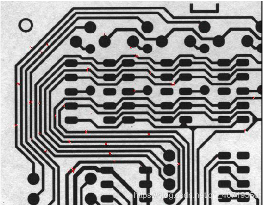
Overview: The basic analysis process of scratch detection consists of two steps: first, determine whether there are scratches on the surface of the inspected product; second, after confirming that scratches exist on the analyzed image, extract the scratches. Due to the diversity of images in industrial inspection, various methods must be considered for each type of image to achieve effective results. Generally, the grayscale value of the scratched area is darker compared to the surrounding normal areas, meaning the grayscale value of the scratched area is lower, and most scratches occur on smooth surfaces, so the overall grayscale variation of the entire image is very uniform, lacking texture features. Basic Methods: Use statistical grayscale features or threshold segmentation methods to highlight the scratched areas.
Source: New Machine Vision