

Click the blue text above to easily follow us.
When analyzing whether there is a correlation between two categorical variables (such as gender and blood type), one might think of using the chi-square test. However, when studying the relationships among 4 or 5 categorical variables simultaneously, the chi-square test becomes insufficient, as it cannot provide a systematic and comprehensive evaluation of the relationships among multiple categorical variables, nor can it estimate the effects of the variables while controlling for other factors. In this case, a log-linear model can be used to study the relationships among multiple variables.[1]
Problems and Data
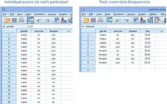
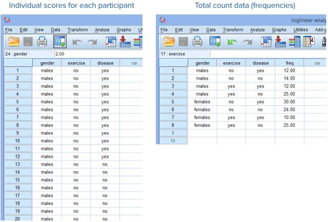
A researcher intends to explore the relationship between gender, physical exercise, and the incidence of heart disease. The researcher has recruited 152 subjects and collected data on whether the subjects participate in physical exercise (yes vs. no), gender (males vs. females), and the incidence of heart disease (yes vs. no), among other related variables. After categorizing and summarizing the data, part of the data is as follows:
Analysis of the Problem
If the researcher intends to analyze the correlation among multiple categorical variables, such as determining the relationship between the subjects’ gender, physical exercise, and the incidence of disease in this study, we can use the log-linear model (loglinear analysis), but four assumptions must first be met:
Assumption 1: All variables are categorical variables, such as the subjects’ gender, participation in physical exercise, and the incidence of heart disease in this study, which are all categorical variables.
Assumption 2: Any expected frequency must be greater than 1, and 80% of expected frequencies must be greater than 5.
Assumption 3: There are no significant outliers.
Assumption 4: The residuals are close to a normal distribution.
After analysis, the data in this study satisfies Assumption 1. So how do we test Assumptions 2-4 and perform log-linear analysis?
SPSS Operations
3.1 Data Weighting
Before performing the official operations, we need to weight the data (for summarized data) as follows:
(1) Click Data → Weight Cases on the main page
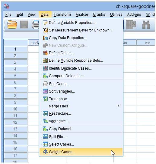
The following dialog box will pop up:
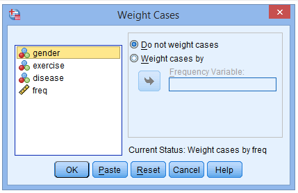
(2) Click on Weight cases by to activate the Frequency Variable window

(3) Place the freq variable into the Frequency Variable field
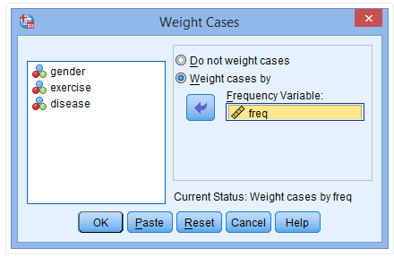
(4) Click OK
3.2 Model Selection
Before running the log-linear model, we need to select a model. Specifically, we mainly determine the number of interaction terms to retain based on the results output by SPSS, ensuring that the accuracy of the data results is not affected. The specific operations are as follows:
(1) Click Analyze → Loglinear → Model Selection on the main interface
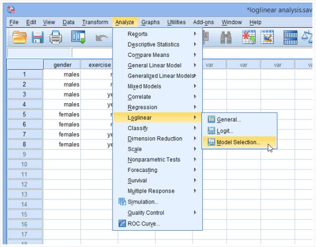
The following dialog box will pop up:
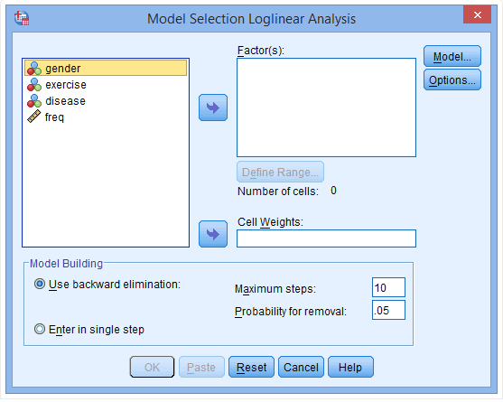
(2) Place the variables gender, exercise, and disease into the Factor(s) field
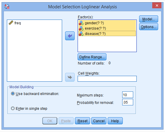
(3) Click on the gender variable to pop up the Define Range field
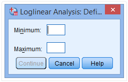
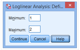
Explanation: In the Define Range field, you should fill in the value range of the corresponding variable. For instance, in the gender variable, “male” is coded as 1 and “female” is coded as 2. Therefore, the minimum value should be filled in as “1” and the maximum value should be filled in as “2”.
(4) Fill in “1” in the Minimum field and “2” in the Maximum field
(5) Click Continue, repeat steps 3-5 to assign value ranges for the exercise and disease variables. Then click Options, and the following dialog box will pop up:
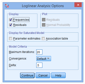
(6) Click on the Parameter estimates and Association table options in the Display for Saturated Model field
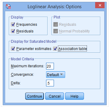
(7) Click Continue → OK
After the above operations, the SPSS output results are as follows:
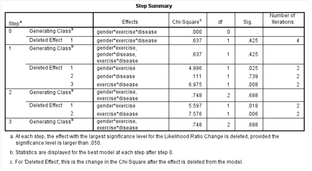
The Step Summary table calculates higher-level interaction terms to lower-level interaction terms step by step from the data.
For example, in this study, there are three variables, so the highest-level interaction term is the gender*exercise*disease interaction, which is “Step 0”. From the Sig column, we can see that after removing the gender*exercise*disease interaction term, P = 0.425, indicating that removing this interaction term does not significantly affect the data results, meaning that this interaction term does not need to be included in the model.
In Step 1, SPSS outputs the calculation results of the lower-level interaction terms, namely gender*exercise, gender*disease, and exercise*disease. Generally, if the results do not show significant differences after removing an interaction term, that is, P > 0.05, we consider that the interaction term can be removed.
In Step 2, SPSS outputs the calculation results after removing the gender*disease interaction term, where the P value for the gender*disease interaction term is 0.739, indicating that this interaction term does not need to be included in the model. The results show that after removing the gender*exercise and exercise*disease terms, the P value is less than 0.05, indicating that these two interaction terms should be included in the model.
Thus, this study should include the gender*exercise and exercise*disease interaction terms, along with the main variables gender, exercise, and disease.
3.3 Log-Linear Analysis Operations
After selecting the model, we need to rerun the log-linear analysis. The specific SPSS operations are as follows:
(1) Click Analyze → Loglinear → General on the main interface
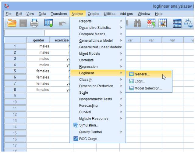
The following dialog box will pop up:
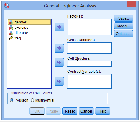
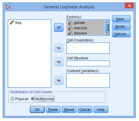
(2) Place the variables gender, exercise, and disease into the Factor(s) field
(3) Click on the Model option
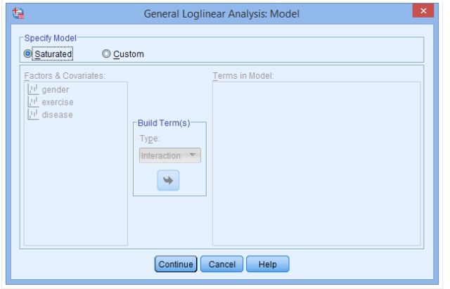
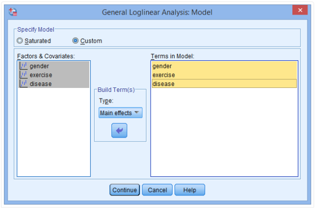
(4) Click Custom in the Specify Model field, and place the gender, exercise, and disease variables from the Factors & Covariates field into the Terms in Model field
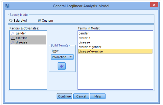
(5) In the Build Term(s) field, select the Interaction option to create the interaction terms for the gender and exercise variables, and the exercise and disease variables as follows:
(6) Click Continue → Options
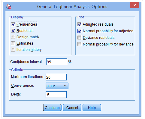
(7) Select the Estimates option in the Display field and fill in “0” in the Delta box in the Criteria field
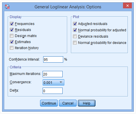
(8) Click Continue → OK
Hypothesis Testing
-
Assumption 2: Any expected frequency must be greater than 1, and 80% of expected frequencies must be greater than 5
After the above operations, the SPSS output of the expected frequency results is as follows:
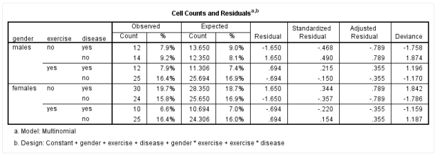
From the Expected column, it can be seen that in this study, the minimum expected frequency is 10.694, indicating that any expected frequency is greater than 1, and 80% of expected frequencies are greater than 5, thus satisfying Assumption 2.
-
Assumption 3: There are no significant outliers
We determine data outliers based on the adjusted residuals, and the SPSS output results are as follows:

Generally, if the adjusted residuals are greater than ±1.96 standard deviations, it indicates that there are outliers in the data. From the Adjusted Residual column, we can see that the largest standardized residuals in this study are 0.789 and -0.789, both of which are less than ±1.96 standard deviations (the standard deviation value needs to be calculated based on the specific data, which will not be elaborated here). According to the table above, all residual values in this study are less than 1.96 standard deviations, thus satisfying Assumption 3.
-
Assumption 4: Residuals are close to a normal distribution
The normal Q-Q plot output based on the adjusted residuals from SPSS is as follows:
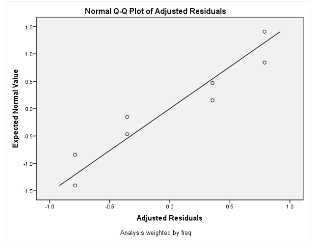
The closer the points on the normal Q-Q plot are to the diagonal line, the closer the data is to a normal distribution; if the points fall exactly on the diagonal, then the data is normally distributed. Log-linear analysis only requires that the adjusted residuals are close to a normal distribution, so based on the above graph, we believe this study satisfies Assumption 4.
Results Interpretation
Before performing log-linear analysis, we need to have a basic understanding of the study data, and the SPSS output results are as follows:
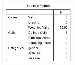
From the Valid row in the table above, we can see that this study has a total of 8 data points, with no missing values (Missing row). This is the result after data weighting, not the information corresponding to the 152 subjects.
From the Goodness-of-Fit Tests table, we can see the fit of the log-linear analysis model as follows:
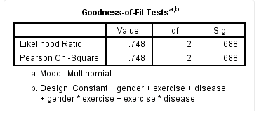
SPSS outputs both the likelihood ratio test and Pearson chi-square test results for model fit in this table. When the sample size is large, the results of these two tests are generally consistent, as in this study where the results of the likelihood ratio test and Pearson chi-square test are the same. However, if the sample size is small, there may be significant differences between the two tests, in which case we recommend using the likelihood ratio test to assess model fit.
Generally speaking, if the predicted frequencies are close to the observed frequencies, the model fit is good, and the test results will indicate a small chi-square value and a large P value. That is, when the test results show P > 0.05, it indicates good model fit, and the results are accurate. However, if the test results show P < 0.05, it indicates that the model fit is poor and suggests that the model should be adjusted appropriately and the log-linear analysis should be redone.
From the table above, the likelihood ratio test results for this study show χ2(2) = 0.748, P = 0.688, indicating that the model fit is good.
The Parameter Estimates table shows the correlation coefficients between the variables as follows:
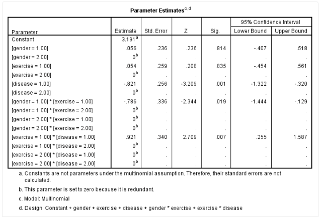
The table does not display the parameters for all variables. For example, for the gender variable, when using females (gender=2.00) as a reference, the coefficient for males (gender=1.00) is 0.056, and the Sig. column indicates whether the coefficient for this variable is statistically significant. The P value for gender is 0.814, which is greater than 0.05, indicating that there is no statistically significant difference between the gender coefficient and 0.
Similarly, for the gender*exercise interaction term, when using [gender=1.00] * [exercise=2.00], [gender=2.00] * [exercise=1.00], and [gender=2.00] * [exercise=2.00] as references, the coefficient for the interaction term for males and non-exercisers [gender=1.00] * [exercise=1.00] is -0.786, P=0.019, indicating that the coefficient for this interaction term is statistically significant. The interpretation of results for other variables is similar and will not be elaborated here.
Writing Conclusions
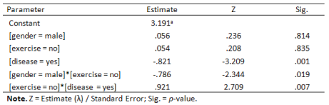
This study uses log-linear analysis to determine the relationship between gender, physical exercise, and the incidence of heart disease. Based on the backward elimination method, the final model includes the three main variables: gender, exercise, and disease, along with the two interaction terms: gender*exercise and exercise*disease. The likelihood ratio test results show χ2(2) = 0.748, P = 0.688, indicating that the model fit is good. The coefficient results suggest that there is a correlation between gender and physical exercise, and that physical exercise is also correlated with the incidence of heart disease (Table 1).
Table 1 Parameter Estimates for the Hierarchical Model (Gender*Exercise, Exercise*Disease)
Further Reading
Some may wonder why not use logistic regression for analysis? There is a very close relationship between log-linear models and logistic regression. The logit process provided in log-linear models can analyze causal relationships between dependent and independent variables, automatically introducing interaction terms between independent and dependent variables into the model. In terms of fitting results, the logit model is actually equivalent to the logistic model.
When it is unclear which of the multiple categorical variables is the cause and which is the result, or when researchers are not interested in the causal relationships between variables but only want to analyze the interactions among variables, log-linear models are typically used instead of logistic regression.[1]
It is worth noting that when too many variables are considered, log-linear models can become overly complex.
References
[1] Zhang Wentong, Chief Editor. Advanced SPSS Statistical Analysis Tutorial.
Explore More Exciting Content
To see more nursing popular science articles related to “Research Fuel Station”, try “In-House Search”! Click the “Protect Your Health” menu below this public account, enter “In-House Search”, and input the keywords you want to search for, such as “Research Fuel Station”, to read related nursing popular science articles!
Source: “Yikahui” Public Account (medieco-ykh)
Author: Li Tongtong
Reprint Format Editor: Zhang Mengjia

If you like it, please click here 👇