What You Must Know About SPICE Models for Circuit Simulation (Part 1)

Today, countless semiconductor chip design companies and design verification engineers use the circuit simulation software SPICE every day. SPICE is widely used in simulating analog circuits (such as operational amplifiers, bandgap reference voltage sources, and AD/DA converters), mixed-signal circuits (such as phase-locked loops, SRAM/dRAM, and high-speed I/O interfaces), precise digital circuits (such as delay, timing, power consumption, and leakage current), establishing timing and power unit libraries for SoCs, analyzing system-level signal integrity, and more. As one of the earliest electronic design automation software, it remains one of the most important software today. It can be said that without SPICE, there would be no electronic design automation industry, and therefore no semiconductor industry as we know it today. Its market exceeds hundreds of millions of dollars. All of this began with a class in the Department of Electrical Engineering at the University of California, Berkeley in 1970.

The Birth of SPICE

Back in 1970, at the University of California, Berkeley’s Department of Electrical Engineering and Computer Sciences (UCBerkeley, Dept. EECS), Professor Ron Rohrer taught a class on “Circuit Synthesis” to seven graduate students. Professor Rohrer had just returned to Berkeley from Fairchild Semiconductor and had no time to prepare teaching materials. So, on the first day of class, he announced: the students would write a circuit simulation program together. He reached an agreement with the department’s teaching director, Professor Don Peterson: as long as Professor Peterson approved the simulation program that the students wrote, they would all pass. Otherwise, they would all fail. One of the seven students had come from the mechanical engineering department and felt very aggrieved: “Professor, I don’t know anything about circuits, I just came to learn about circuits. Now, instead of learning about circuits, I have to write a circuit simulation program. What should I do?” Professor Rohrer thought for a moment and said it was okay. Although you don’t understand circuits, your numerical analysis skills are quite good, right? OK, you are responsible for solving the equations. The final result proved that the module for solving sparse matrices developed by the students was a highlight, allowing the processable circuit scale to increase exponentially. Why do I say this? If you have studied numerical methods, you know that the Gaussian elimination method is generally used to solve systems of equations. Its complexity is O(n^3). This means that if the circuit scale doubles, your computation time increases to 8 times. At that time, the circuit simulation program could simulate at most 10 transistors. Exceeding this number would either burn out your budget or exhaust your patience. However, the students noticed that the matrices generated from the circuits had a characteristic of sparsity: many elements in a circuit matrix are 0 (indicating that there is no connection between two circuit nodes). Since they are 0, there is no need to store and compute them. This significantly reduced both storage and computation (even elementary school students know that any number multiplied by 0 is still 0. So, don’t engage in a lot of unnecessary multiplications by 0).

Many of the basic elements in SPICE originated from this circuit analysis class project guided by Professor Rohrer, including the sparse matrix solving module mentioned above and the use of implicit integration algorithms, which made transient analysis more stable. Additionally, the program included built-in semiconductor device models, allowing users to provide only a set of model parameters without needing to supply their own device model FORTRAN modules.

The seven students elected Laurence Nagel as their representative to report the results to Professor Peterson. The result was named CANCER. Yes, it means “Cancer”. It is the abbreviation for “Computer Analysis of Nonlinear Circuits, Excluding Radiation”. Don’t forget, this was during a rebellious era. At that time, most circuit analysis software was developed under contracts with large companies and the government/military. In the context of the Cold War and nuclear threats, the government/military required that these software be capable of analyzing circuits’ resistance to nuclear radiation. Berkeley was a stronghold of anti-war sentiment, and the program developed by the students was naturally designed to oppose the government/military’s requirements.

Some students might ask: why develop a circuit simulation program? Well, before this, people analyzed circuits either with pen and paper or by building circuit boards (breadboards). Professor Peterson was referred to by the students as the “envelope professor” because he thought that analyzing circuits on the back of an envelope was sufficient. However, as circuit scales increased, using pen and paper became increasingly impractical, and building circuit boards could not accurately reflect the characteristics of circuits on chips, not to mention the rising costs. Therefore, the urgency to use software for circuit simulation became increasingly apparent.

When the course ended, after Nagel reported CANCER to Professor Peterson, Professor Peterson fully recognized it. All the students passed! CANCER became Nagel’s master’s thesis topic. It was used by many undergraduate and graduate students at Berkeley and received extensive suggestions for improvement. It is often said that students are the best “guinea pigs,” and this statement proved to be true (to add a note: based on the huge success of this class, Professor Rohrer later tried a few more classes using the same method, but all failed. He summarized that it was because of Nagel that the Berkeley class succeeded. So, without a professor like Rohrer and a talented student like Nagel, SPICE could not have been born from a single class).

By the fall of 1971, Nagel began his doctoral studies at Berkeley, this time under the guidance of Professor Peterson. (Before this, Professor Rohrer had left Berkeley for industry. The reason was that Professor Rohrer and Professor Peterson had different opinions on whether to make CANCER’s source code public. Professor Rohrer later returned to academia as a professor at Carnegie Mellon University (CMU) and guided the development of AWE, but that’s a different story.)

Professor Peterson’s first task for Nagel was to give the program a new name. Indeed, CANCER is too unpleasant; no one likes it. Nagel spent who knows how long coming up with a name that is pleasant and that we still use today: SPICE (Simulation Program with Integrated Circuit Emphasis). (So, students, if you are going to write a new program, start a new company, or name a child, be sure to give her/him a nice name.) The year 1971 was officially recognized as the year of SPICE’s birth.

Nagel’s photo from that year at Berkeley

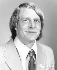
Professor Rohrer

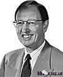
Professor Peterson

SPICE was also a pioneer of open-source code. At that time, there was open-source code, but it had little commercial value. SPICE was different. Some had already seen its commercial value, but Professor Peterson insisted on making the code open-source (we should sincerely thank Professor Peterson). Anyone could obtain the source code of SPICE for a $20 handling fee (of course, during the Cold War, SPICE was prohibited from being exported to countries deemed “communist” by the government). Some might ask: did Berkeley lose a lot of money this way? Not at all. Berkeley’s SPICE helped Digital Equipment Corporation (DEC) sell many VAX machines. In return, DEC donated $18 million to Berkeley’s electrical engineering department (considering inflation, you can imagine how much that is worth today). This amount of money is not something a school could earn by selling code. So, doing good ultimately brings good rewards.

SPICE2 and SPICE3

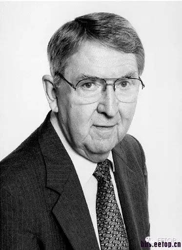
In the early 1970s, Berkeley’s electrical engineering department used the CDC 6400 mainframe, which had computing power equivalent to a 286 (with a clock frequency of 10 MHz, costing six million dollars. Compare this to today’s iPhone, which has a clock frequency exceeding 1000 MHz and costs less than six hundred dollars – that’s a million-fold difference in cost-performance!). Each student had a main memory of 256K bytes during the day. At night, when there were fewer people, you could get 384K. Running a not-too-large circuit simulation, in Nagel’s words, was like putting your size 11 foot into a baby’s shoe – you had to think of every possible way to save memory. The maximum circuit size that could be simulated was about 25 bipolar transistors (equivalent to 50 circuit nodes). At that time, SPICE only had bipolar transistor models. In the fall of 1971, Professor David Hodges, who came to Berkeley from Bell Labs, brought the first MOSFET model: the Shichman-Hodges model. If you’ve used SPICE (and have been around long enough), you should know this is the Level 1 MOSFET model, the ancestor of all MOSFET models (which we will discuss later).

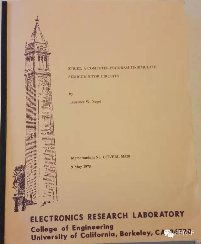
In 1975, Nagel graduated with his PhD from Berkeley. His thesis, “SPICE2: A COMPUTER PROGRAM TO SIMULATE SEMICONDUCTOR CIRCUITS,” became the most cited paper in the EDA industry.

The SPICE2 version basically laid the foundation for today’s circuit simulation programs, including: improved nodal analysis (Modified Nodal Analysis), sparse matrix solving (Sparse Matrix Solver), Newton-Raphson iteration (Newton-Raphson Iteration), implicit numerical integration (Implicit Numerical Integration), dynamic time step control (Dynamic Time Step Control), local truncation error (Local Truncation Error), etc. – too many technical details, let’s continue with the story.

After graduating, Nagel went to Bell Labs. From then on, the improvements to SPICE2 were continued by Nagel’s roommate, Ellis Cohen, who was a programming expert. As the students around him said, he was like a human-shaped computer. He (along with later contributors Andrei Vladimirescu and Sally Liu) transformed the program developed at the school into a practical SPICE2G6. In the early development of SPICE, he was an unsung hero. Many commercial SPICE programs in the industry today are based on SPICE2G6.

This is the cover of Nagel’s doctoral thesis.

You can download this thesis using the link below:

http://www.eecs.berkeley.edu/Pubs/TechRpts/1975/9602.html

If you want to understand the core secrets of SPICE, download it and read it carefully!

The earliest SPICE2 had no user interface. It ran in batch mode. This means that once you prepared your circuit description and simulation commands, you would submit them to the host system. Then what? Then you could go home (how nice!). Because your dozens (or hundreds) of colleagues were doing the same thing. It was like having only one clerk (the host) in a bank, while hundreds of customers (the submitted simulation tasks) were queuing up. And that clerk was slow (286 speed). So, you would have to wait until the next morning to see the results! (We will discuss this situation further when we talk about HSPICE).

The input for SPICE2 was done using punched cards. You might ask: what are punched cards? Well, congratulations, you are young enough. For those over fifty, the first computer input interface they encountered looked like this:

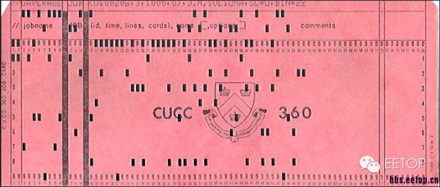
You would type your circuit description and simulation commands on a stack of such cards and put them into a card reader. You may have heard that SPICE’s input is called a “SPICE DECK”; this name comes from this stack of cards.

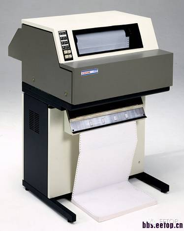
The output of SPICE2 was produced by line printers. Yes, it printed simulation results on paper using printers like the one below (imagine how much paper was consumed at that time).

You could also print input/output signal waveforms. Each waveform was drawn using different characters. Like the image below (doesn’t it look quite rough?):

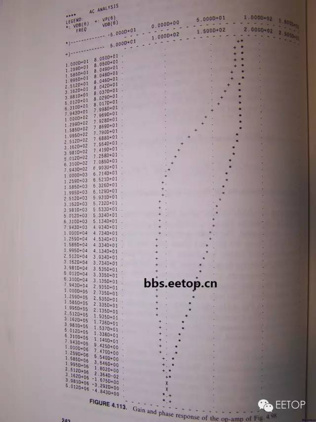
Some students reading the SPICE manual might see a strange option called “NOPAGE.” This is because SPICE’s output would insert a page break between pages, leaving a blank space. This option requests not to stop printing. This way, waveforms would not be interrupted between pages. As line printers became obsolete, this option also entered history. Hehe, if anyone knows this option, they must be at least 40 years old.

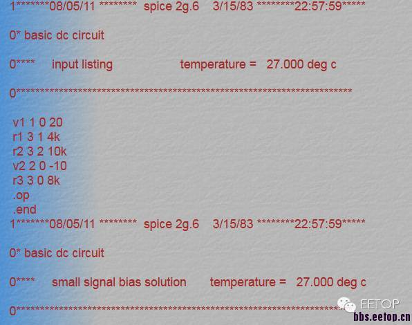
Later, SPICE2’s input/output evolved into file input/output, like the one below:

By the 1980s, SPICE2 had spread throughout various universities. However, its problems also became apparent: FORTRAN code was too difficult to maintain, and adding new device models required too many changes, etc. At the same time, C as a new programming language was gaining popularity. Therefore, rewriting SPICE in C was put on the agenda. This task was completed by Thomas Quarles from Berkeley in 1989. Compared to SPICE2, SPICE3 added a user interface, allowing you to use commands and even command strings to control the program. Moreover, it also included a graphical interface for viewing waveforms. More importantly, SPICE3’s program architecture became clearer and more modular, making it easier to maintain and modify. The 1980s also saw explosive advancements in computer hardware: mainframes were replaced by workstations. UNIX and the C-shell and X-window built on it became the basic framework for software development and applications. Additionally, personal computers (PCs) became increasingly popular. All of these laid a solid foundation for the widespread application of SPICE (which we will discuss when talking about commercial SPICE).

This is the cover of Quarles’ thesis:

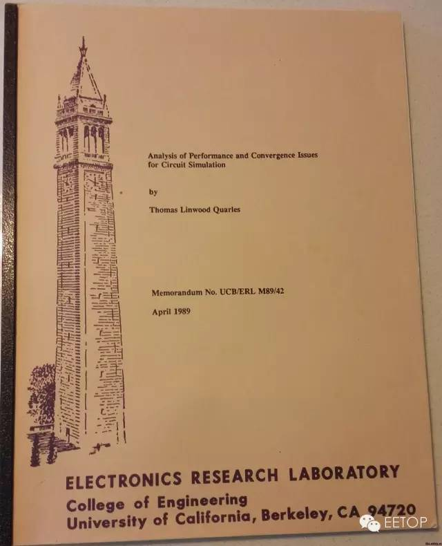
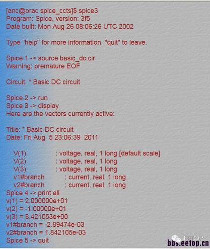
Similarly, you can download Quarles’ thesis using the link below: http://www.eecs.berkeley.edu/Pubs/TechRpts/1989/ERL-89-46.pdf Below is the execution statement for SPICE3 (version 3f5). Note that it is interactive. Each “Spice->” is followed by a SPICE3 command. For example, “source” reads in the circuit, “run” executes it, “display” shows it, and “quit” exits.

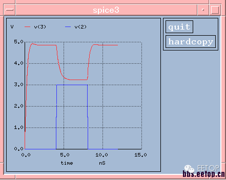
SPICE3 comes with a graphical module called nutmeg. Below is the waveform displayed by nutmeg. Isn’t it much better looking than the character waveforms printed by SPICE2?

Since the 1990s, the development of SPICE in academia has basically stagnated at SPICE3f5. Does this mean that SPICE has stagnated? Not at all. SPICE has continued to evolve in at least two directions: one is device models (especially MOSFET models), and the other is commercial SPICE programs. (It is worth mentioning that a group of SPICE enthusiasts and universities took SPICE3f5 and integrated it with several other open-source software (xspice, cider, gss, adms, etc.) to create ngspice. Ngspice is also evolving slowly, but its pace is much slower than that of commercial SPICE programs. You can find ngspice on sourceforge.)