Official WeChat account of Tsinghua Big Data Software Team
Source: Zhihu

This article is about 5000 words long, and it is recommended to read for 5 minutes.
This article systematically summarizes the related content about decision trees, random forests, etc.
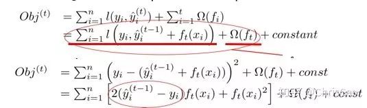
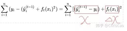
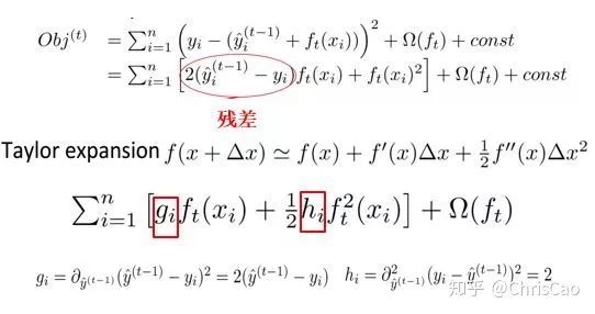
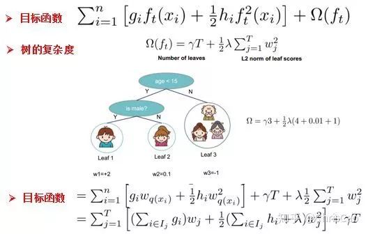
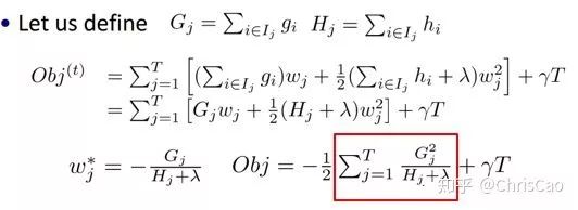
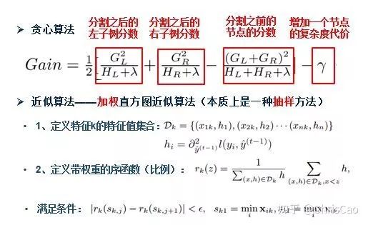
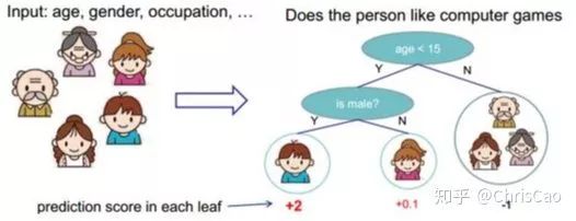
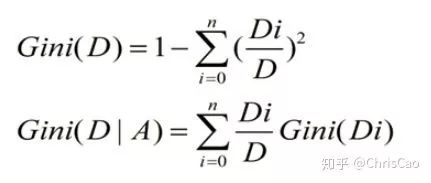
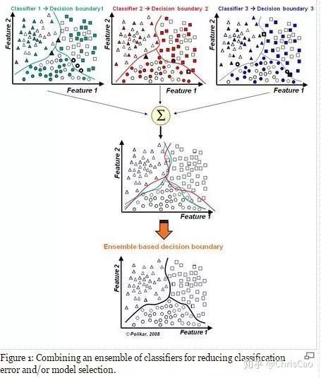
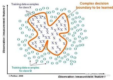
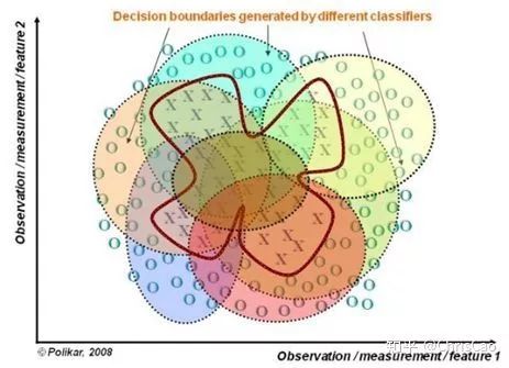
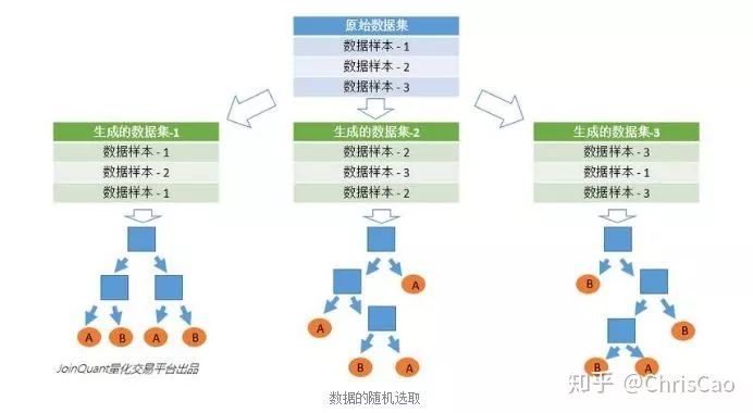
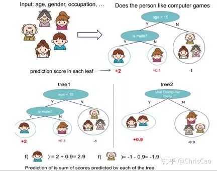
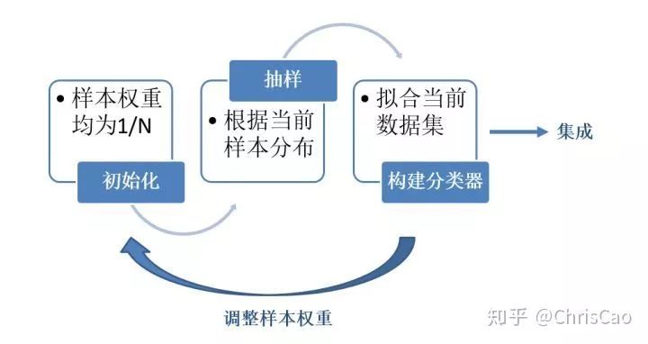
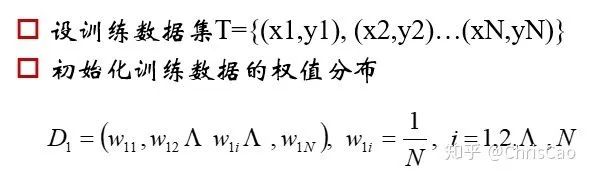
1、Decision TreeA decision tree is a supervised classification model that essentially selects a feature value with the maximum information gain for splitting the input until the stopping condition is met or the purity of the leaf nodes reaches the threshold. The diagram below is an example of a decision tree:According to the splitting criteria and methods, decision trees can be divided into: ID3, C4.5, and CART algorithms.1. ID3 Algorithm: Selects the Optimal Partition Attribute Based on Information GainThe calculation of information gain is based on information entropy (a measure of the purity of a sample set). The smaller the information entropy, the greater the purity of the dataset .Assuming a decision tree is built based on the dataset with categories:In formula (1): represents the proportion of the total number of samples of class K to the total number of samples in dataset D.Formula (2) indicates that using feature A as the splitting attribute results in the information entropy: Di represents the set of nodes in the i-th branch formed by partitioning by attribute A. Thus, this formula calculates the total information entropy of n branches formed by partitioning by attribute A.Formula (3) is the difference in information entropy before and after partitioning by A, which is the information gain, the greater the better.Assuming each record has an attribute ‘ID’, if we partition based on ID, the feature values that can be obtained on this attribute are the sample counts. If the number of features is too large, regardless of which ID is used for partitioning, the leaf node values will only have one, resulting in high purity and large information gain. Thus, the decision tree formed this way is meaningless, i.e., ID3 tends to favor attributes with many values for partitioning, which has a certain bias. To reduce this effect, some scholars proposed the C4.5 algorithm.2. C4.5: An Algorithm that Selects the Most Optimal Partition Attribute Based on Information Gain RatioInformation gain ratio introduces a penalty term known as split information to penalize attributes with many values:, Where IV(a) is determined by the number of feature values of attribute A; the more values, the larger the IV value, the smaller the information gain ratio, thus avoiding the model’s preference for attributes with many feature values. If we simply split according to this rule, the model will prefer attributes with fewer feature values. Therefore, C4.5 first identifies candidate partition attributes with information gain above average, and then selects the one with the highest gain ratio from them.For continuous value attributes, the number of possible values is no longer limited, so discretization techniques (such as binary methods) can be used. The attribute values are sorted from smallest to largest, and the median value is selected as the split point; points with values smaller than it are assigned to the left subtree, and points not smaller than it are assigned to the right subtree, and the information gain ratio of the split is calculated, selecting the attribute value with the highest information gain ratio for splitting.3. CART: Selects the Optimal Partition Attribute Based on Gini Index, Can Be Used for Classification and RegressionCART is a binary tree that uses binary splitting; it splits the data into two parts each time, entering the left and right subtrees respectively. Each non-leaf node has two children, so the leaf nodes of CART are one more than the non-leaf nodes. Compared to ID3 and C4.5, CART is applied more widely, as it can be used for both classification and regression. In CART classification, the Gini index is chosen as the best classification feature, which describes purity and has a meaning similar to information entropy. In CART, the Gini coefficient is reduced at each iteration.Gini(D) reflects the purity of dataset D; the smaller the value, the higher the purity. We select the attribute that minimizes the Gini index after partitioning from the candidate set as the optimal partition attribute.Classification Tree and Regression TreeFirst, let’s discuss classification trees. ID3 and C4.5 exhaustively check each threshold of each feature attribute at each branch to find the feature that maximizes the entropy of the two branches formed by the feature values <= threshold and feature values > threshold. This standard branching creates two new nodes, and the same method is applied until all individuals are assigned to a uniquely gendered leaf node or the preset stopping condition is met. If the final leaf node does not have a unique gender, the majority gender is assigned to that leaf node.The overall process for regression trees is similar, but at each node (not necessarily a leaf node), a predicted value is obtained. For example, the predicted value for age equals the average age of all individuals in that node. During branching, every threshold of each feature is exhaustively checked to find the best split point, but the measure used is to minimize the mean squared error, i.e., the total of (each individual’s age – predicted age)^2 / N, or the sum of the squared prediction errors for each individual divided by N. This is understandable; the more individuals predicted to be coarse, the more outrageous the errors, resulting in a larger mean squared error. By minimizing the mean squared error, we find the most reliable basis for branching. Branching continues until the ages of individuals at each leaf node are unique (which is very difficult) or until the preset stopping condition (such as a limit on the number of leaves) is reached. If the final leaf node does not have a unique age, the average age of all individuals in that node is used as the predicted age for that leaf node.2、Random ForestFirst, let’s supplement the concept of ensemble classifiers, which combine the results of multiple classifiers through voting or averaging to arrive at the final result.1. Benefits of Building Ensemble Classifiers:(1) Improve model accuracy: Integrating the classification results of various models leads to a more reasonable decision boundary, reducing overall errors and achieving better classification results:(2) Handle overly large or small datasets: When the dataset is large, it can be divided into multiple subsets to build classifiers for each subset; when the dataset is small, bootstrap sampling can be used to create multiple different datasets from the original dataset to build classifiers.(3) If the decision boundary is too complex, linear models cannot accurately describe the true situation. Therefore, for datasets in specific regions, multiple linear classifiers are trained, and then they are integrated.(4) More suitable for handling multi-source heterogeneous data (different storage methods (relational, non-relational), different categories (time series, discrete, continuous, network structure data))Random forests are a combination classifier of multiple decision trees, where randomness is mainly reflected in two aspects: the randomness of data selection and the randomness of feature selection.(1) Random selection of dataFirst, bootstrap sampling is performed from the original dataset to construct a subset, with the number of elements in the subset being the same as that in the original dataset. Elements in different subsets can be repeated, and elements within the same subset can also be repeated.Second, using the subset to build sub-decision trees, this data is input into each sub-decision tree, and each sub-decision tree outputs a result. Finally, if new data needs to be classified by the random forest, the voting results from the sub-decision trees are used to obtain the output result of the random forest. As shown in the figure below, if there are 3 sub-decision trees in the random forest, with 2 trees classifying it as class A and 1 tree classifying it as class B, then the classification result of the random forest is class A.(2) Random selection of candidate featuresSimilar to random selection of datasets, during the splitting process of each subtree in the random forest, not all candidate features are used; rather, a certain number of features are randomly selected from all candidate features, and then the optimal feature is chosen from the randomly selected features. This allows the decision trees in the random forest to differ, enhancing the diversity of the system, thereby improving classification performance.Example diagram of ensemble trees3. GBDT and XGBoost1. Before discussing GBDT and XGBoost, let’s supplement knowledge on Bagging and Boosting.Bagging is a parallel learning algorithm with a simple idea: each time, a dataset of the same size is sampled from the original data based on a uniform probability distribution with replacement. Sample points can appear multiple times, and a classifier is constructed for each generated dataset, which are then combined.Boosting has different sample distributions for each sampling; at each iteration, the weights of misclassified samples are increased based on the results of the previous iteration. This causes the model to pay more attention to difficult-to-classify samples in subsequent iterations. This is a continuous learning process and a continuous improvement process, which is the essence of the Boosting idea. After iteration, the base classifiers from each iteration are integrated, and how to adjust sample weights and integrate classifiers is a key issue we need to consider.Structure diagram of Boosting algorithmTaking the famous Adaboost algorithm as an example:There is a dataset with a sample size of N, each sample corresponds to an original label. Initially, we set the weights of the samples to 1/N. The classification error rate of the model is calculated based on the current data, and the coefficient value of the model is based on the classification error rate.According to the model’s classification results, the distribution of data in the original dataset is updated, increasing the probability of misclassified data being sampled so that they can be retrained by the model in the next iteration.The final classifier is a combination of all base classifiers.2. GBDTGBDT is a gradient boosting algorithm using decision trees (CART) as base learners, and it is an iterative tree rather than a classification tree. Boost means “enhancement”; generally, Boosting algorithms are iterative processes where each new training aims to improve upon the previous results. With the previous explanation of Adaboost, the general idea should be easy to understand.The core of GBDT is: each tree learns the residuals of the conclusions from all previous trees. This residual is the accumulated amount that, when added to the predicted value, gives the true value. For example, if A’s true age is 18 years, but the first tree predicts A’s age as 12 years, the residual is 6 years. Therefore, in the second tree, we set A’s age to 6 years for learning, and if the second tree can indeed place A in the leaf node for 6 years, then the accumulated conclusions from the two trees will equal A’s true age. If the conclusion from the second tree is 5 years, then A still has a residual of 1 year, and in the third tree, A’s age will be adjusted to 1 year for further learning.3. XGBoostXGBoost applies numerical optimization more effectively than GBDT, and most importantly, the loss function (the error between predicted values and true values) becomes more complex. The objective function is still the sum of the predicted values from all trees equaling the predicted value.The loss function is as follows, introducing first and second derivatives:A good model needs to have two basic elements: one is good accuracy (i.e., good fitting), and the other is that the model should be as simple as possible (complex models are prone to overfitting and are less stable). Therefore, the right side of the objective function we constructed has the first term as the error term of the model, and the second term as the regularization term (which penalizes model complexity).Common error terms include squared error and logistic loss, while common regularization terms include L1 and L2 regularization. L1 regularization sums the model’s elements, while L2 regularization squares the elements.In each iteration, a new tree is added to fit the residuals between the predictions of the previous trees and the true values.The objective function is as shown in the figure, and the last row’s circled part is essentially the residual between the predicted and true values.First, let’s expand the training error:XGBoost performs a second-order Taylor expansion on the cost function while using the first and second derivatives of the sum of squared residuals.Next, let’s investigate the regularization term in the objective function:The complexity of a tree can be measured by the number of branches, which can be represented by the number of leaf nodes.Thus, the complexity of the tree is expressed as: the first term on the right is the number of leaf nodes T, and the second term is the L2 regularization of the weights w of the tree’s leaf nodes, which prevents excessive leaf nodes.At this point, in each iteration, we effectively add a tree to the existing model. In the objective function, we denote a tree by wq(x), which includes the structure of the tree and the weights of the leaf nodes. Here, w represents the weights (reflecting prediction probabilities), and q represents the index of the sample (reflecting the tree’s structure).By deriving the final objective function with respect to parameters w and substituting it back into the objective function, we can see that the value of the objective function is determined by the part marked in red:Therefore, the iterations of XGBoost are defined by the gain formula shown in the figure below, which is used to select the optimal split point:So how do we obtain an excellent ensemble tree?One method is the greedy algorithm, which traverses all features within a node, calculates the information gain for each feature based on the formula, and finds the point with the highest information gain for tree splitting. The new leaf penalty corresponds to tree pruning; when the gain is below a certain threshold, we can prune this split. However, this method is not suitable for large datasets, so we need to use approximate algorithms.Another method: XGBoost does not enumerate all feature values when searching for split points, but performs aggregated statistics on feature values, constructing histograms to compute the area of feature value distributions, then forming several buckets with equal areas. The feature values on the boundaries of the buckets are treated as candidates for split points.The explanation of the approximate algorithm formula in the figure: sorting the feature k’s values, calculating the distribution of feature values, rk(z) represents the proportion of the total weight for feature k that is less than z, indicating the importance of these feature values. We calculate the formula based on this proportion, dividing the feature values into several buckets with equal proportions, selecting the boundaries of these feature values as candidate split points, forming a candidate set. The condition for selecting the candidate set is that the difference between two adjacent candidate split nodes must be less than a certain threshold.Based on the above, we can summarize the innovations of XGBoost compared to GBDT:1. Traditional GBDT uses CART as the base classifier, while XGBoost also supports linear classifiers, making it equivalent to logistic regression (for classification problems) or linear regression (for regression problems) with L1 and L2 regularization terms.2. Traditional GBDT only uses first-order derivative information during optimization, while XGBoost performs a second-order Taylor expansion on the cost function, utilizing both first and second derivatives. It is worth mentioning that the XGBoost tool supports custom cost functions as long as they can be derived first and second order.3. XGBoost incorporates regularization terms into the cost function to control model complexity. These regularization terms include the number of leaf nodes in the tree and the square of the L2 norm of the output scores for each leaf node. From the perspective of the bias-variance tradeoff, the regularization term reduces the model’s variance, resulting in a simpler learned model that prevents overfitting, which is another feature that makes XGBoost superior to traditional GBDT.4. Shrinkage, equivalent to the learning rate (eta in XGBoost). In each iteration, a new model is added, with a coefficient less than 1 applied to the previous model, reducing the optimization speed. Taking smaller steps to approach the optimal model is easier to avoid overfitting than taking large steps.5. Column subsampling. XGBoost borrows from the practices of random forests, supporting column subsampling (i.e., not using all features for each input). This not only reduces overfitting but also decreases computation, which is another feature that distinguishes XGBoost from traditional GBDT.6. Ignoring missing values: When searching for split points, samples with missing values for that feature are not traversed for statistics; only the feature values corresponding to non-missing samples are traversed, reducing the time cost of finding split points for sparse discrete features.7. Specifying the direction for missing values: The direction for branches can be specified for missing values or specified values. To ensure completeness, both scenarios are handled where samples with missing feature values are assigned to either the left or right leaf nodes, and the direction leading to the greater gain is chosen as the default direction. This greatly enhances the efficiency of the algorithm.8. Parallel processing: Before training, each feature is pre-sorted to identify candidate splitting points, and stored in a block structure. This structure is reused in subsequent iterations, significantly reducing computational load. During node splitting, the gain for each feature needs to be computed, and the feature with the maximum gain is selected for splitting. Therefore, the gain calculations for various features can be performed in parallel using multiple threads, thereby finding the optimal split point across different feature attributes.Editor: Wang Jing


 The smaller the information entropy, the greater the purity of the dataset
  .
. with
with  categories:
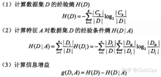
 represents the proportion of the total number of samples of class K to the total number of samples in dataset D.
 ,
, 
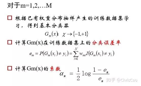
 The classification error rate of the model is calculated based on the current data, and the coefficient value of the model is based on the classification error rate.