Originally from Python Artificial Intelligence Frontier
In simple terms, a machine learning model is a type of mathematical function that maps input data to predicted outputs. More specifically, a machine learning model is a mathematical function that adjusts model parameters through learning from training data to minimize the error between predicted outputs and actual labels.
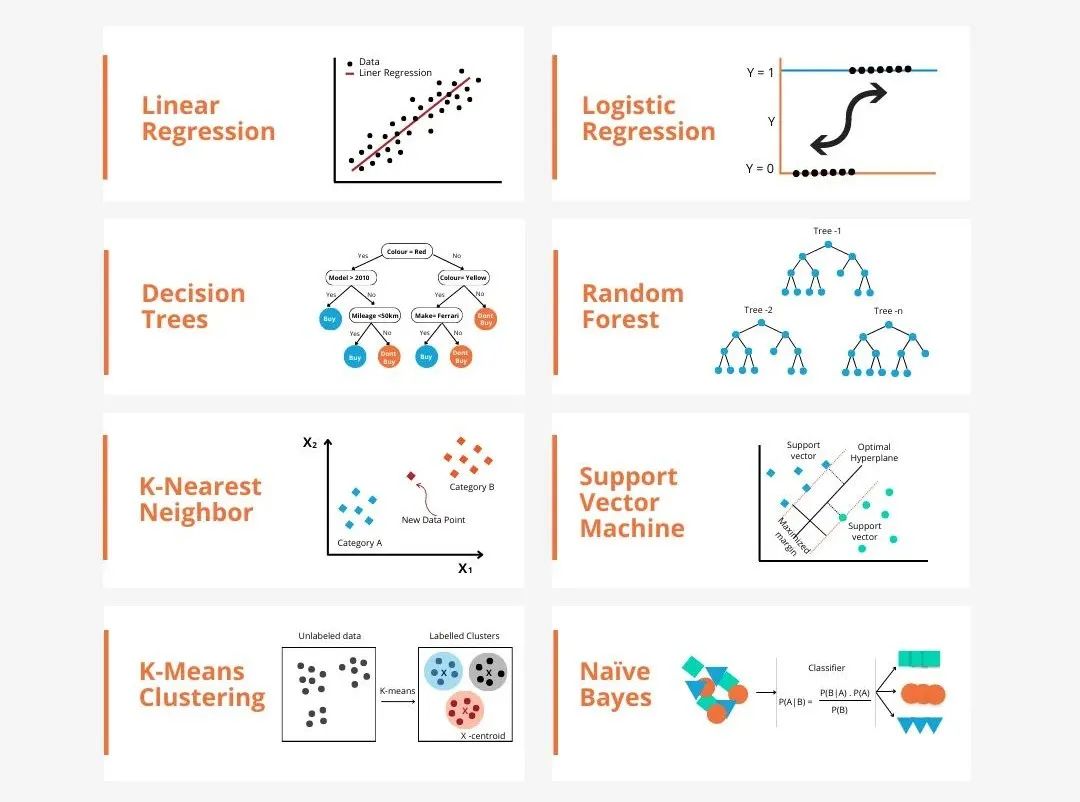
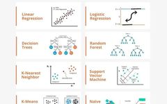
There are many types of models in machine learning, such as logistic regression models, decision tree models, support vector machine models, etc. Each model has its applicable data types and problem types. At the same time, there are many commonalities between different models, or there is a hidden evolutionary path of models.
Taking the connectionist perceptron as an example, by increasing the number of hidden layers in the perceptron, we can transform it into a deep neural network. Adding a kernel function to the perceptron can transform it into an SVM. This process visually demonstrates the intrinsic connections between different models and the potential for transformation between models. Based on similarities, I have roughly (not rigorously) classified the models into the following six major categories to facilitate the discovery of basic commonalities and to analyze them in depth one by one!
1. Neural Network (Connectionist) Models:
Connectionist models are computational models that simulate the structure and function of the human brain’s neural networks. The basic unit is the neuron, which receives inputs from other neurons and adjusts weights to change the influence of inputs on the neuron. Neural networks are black boxes that can achieve universal approximation through multiple layers of nonlinear hidden layers.

The representative models include DNN, SVM, Transformer, and LSTM. In some cases, the last layer of a deep neural network can be viewed as a logistic regression model used to classify input data. Support vector machines can also be seen as a special type of neural network with only two layers: an input layer and an output layer. SVM additionally achieves complex nonlinear transformations through kernel functions, achieving results similar to deep neural networks. The following is an analysis of the classic DNN model principles:

Deep Neural Networks (DNN) consist of multiple layers of neurons that pass input data through each layer of neurons via a forward propagation process, calculating outputs layer by layer. Each layer of neurons receives the output from the previous layer as input and outputs to the next layer of neurons. The training process of DNN is achieved through a backpropagation algorithm. During training, the error between the output layer and the actual labels is computed, and the error is backpropagated to each layer of neurons, updating the weights and biases of the neurons according to the gradient descent algorithm. By repeatedly iterating this process, the network parameters are continuously optimized to minimize the prediction error of the network.
The advantages of DNN include strong feature learning capabilities: DNN can automatically learn features of the data without manual feature design. High nonlinearity and strong generalization ability. The disadvantages are that DNN requires a large number of parameters, which may lead to overfitting problems. Also, DNN has a large computational load and long training time, and the model’s interpretability is weak. The following is a simple Python code example that uses the Keras library to build a deep neural network model:
from keras.models import Sequential  from keras.layers import Dense  from keras.optimizers import Adam  from keras.losses import BinaryCrossentropy  import numpy as np
# Build model  model = Sequential()  model.add(Dense(64, activation='relu', input_shape=(10,))) # Input layer with 10 features  model.add(Dense(64, activation='relu')) # Hidden layer with 64 neurons  model.add(Dense(1, activation='sigmoid')) # Output layer with 1 neuron, using sigmoid activation function for binary classification
# Compile model  model.compile(optimizer=Adam(lr=0.001), loss=BinaryCrossentropy(), metrics=['accuracy'])
# Generate simulated dataset  x_train = np.random.rand(1000, 10) # 1000 samples, each with 10 features  y_train = np.random.randint(2, size=1000) # 1000 labels for binary classification
# Train model  model.fit(x_train, y_train, epochs=10, batch_size=32) # Train for 10 epochs, using 32 samples each time
2. Symbolic Models
Symbolic models are a method of intelligent simulation based on logical reasoning, which considers humans as physical symbol systems, and computers as physical symbol systems. Therefore, we can use a computer’s rule base and inference engine to simulate human intelligent behavior, that is, using computer symbol operations to simulate human cognitive processes (in simple terms, it is storing human logic in a computer to achieve intelligent execution).
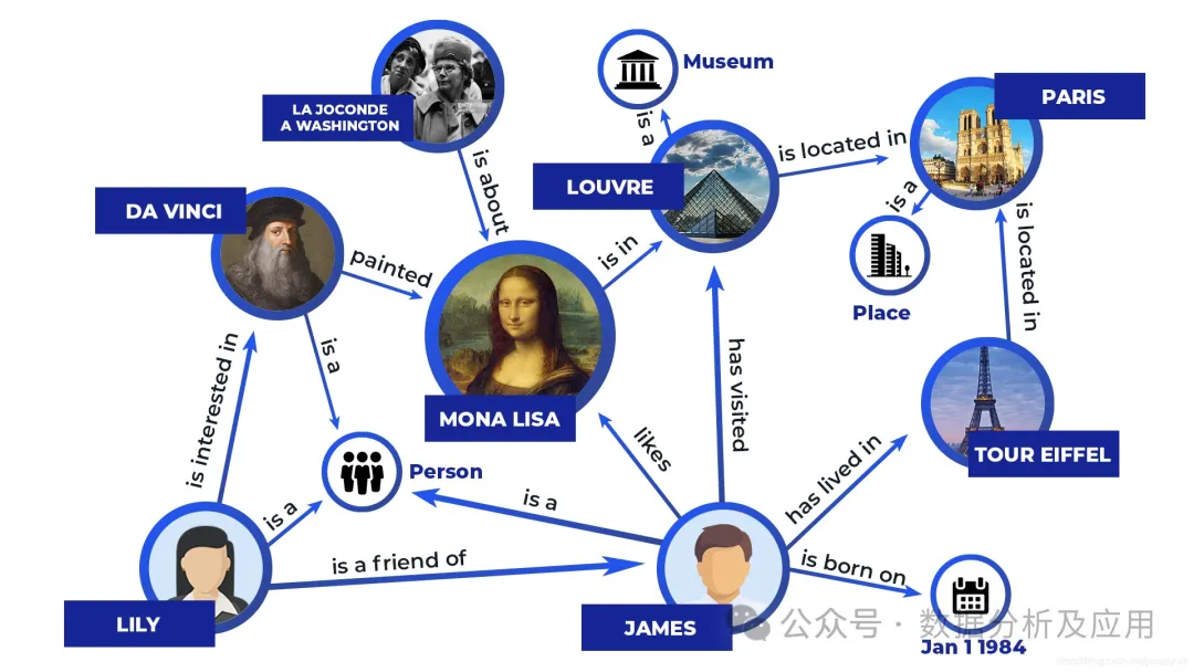
The representative models include expert systems, knowledge bases, and knowledge graphs, which encode information into a set of recognizable symbols and operate on these symbols using explicit rules to produce computational results. Below is a simple example of an expert system:
# Define rule base  rules = [      {"name": "rule1", "condition": "sym1 == 'A' and sym2 == 'B'", "action": "result = 'C'"},      {"name": "rule2", "condition": "sym1 == 'B' and sym2 == 'C'", "action": "result = 'D'"},      {"name": "rule3", "condition": "sym1 == 'A' or sym2 == 'B'", "action": "result = 'E'"},  ]
# Define inference engine  def infer(rules, sym1, sym2):      for rule in rules:          if rule["condition"] == True:  # Execute action when condition is true              return rule["action"]      return None  # Return None when no rule satisfies the condition
# Test expert system  print(infer(rules, 'A', 'B'))  # Output: C  print(infer(rules, 'B', 'C'))  # Output: D  print(infer(rules, 'A', 'C'))  # Output: E  print(infer(rules, 'B', 'B'))  # Output: E
3. Decision Tree Models
Decision tree models are a non-parametric classification and regression method that uses tree diagrams to represent decision processes. More colloquially, the mathematical description of tree models is “piecewise functions.” It uses the entropy theory in information theory to select the best partition attributes for the decision tree to build a decision tree with optimal classification performance.
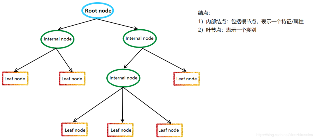
The basic principle of decision tree models is to recursively partition the dataset into several subsets until each subset belongs to the same category or meets a certain stopping condition. During the partitioning process, decision tree models use metrics such as information gain, information gain ratio, and Gini index to evaluate the quality of the partitioning to select the best partition attributes.
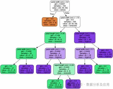
There are many representative models of decision tree models, among which the most famous are ID3, C4.5, and CART. The ID3 algorithm is the ancestor of decision tree algorithms, using information gain to select the best partition attribute; the C4.5 algorithm is an improved version of the ID3 algorithm, using information gain ratio to select the best partition attribute while employing pruning strategies to enhance the generalization ability of the decision tree; the CART algorithm, short for Classification and Regression Trees, uses the Gini index to select the best partition attributes and can handle both continuous and ordinal attributes.
The following is a code example using the CART algorithm implemented in Python’s Scikit-learn library:
from sklearn.datasets import load_iris  from sklearn.model_selection import train_test_split  from sklearn.tree import DecisionTreeClassifier, plot_tree
# Load dataset  iris = load_iris()  X = iris.data  y = iris.target
# Split into training and testing sets  X_train, X_test, y_train, y_test = train_test_split(X, y, test_size=0.2, random_state=42)
# Build decision tree model  clf = DecisionTreeClassifier(criterion='gini')  clf.fit(X_train, y_train)
# Predict results for test set  y_pred = clf.predict(X_test)
# Visualize decision tree  plot_tree(clf)
4. Probabilistic Models
Probabilistic models are mathematical models based on probability theory, used to describe the distribution, occurrence probabilities of random phenomena or events, and the probabilistic relationships between them. Probabilistic models have wide applications in various fields, such as statistics, economics, and machine learning.
The principle of probabilistic models is based on the basic principles of probability theory and statistics. They use probability distributions to describe the distribution of random variables and probability rules to describe the conditional relationships between events. Through these principles, probabilistic models can quantitatively analyze and predict random phenomena or events.
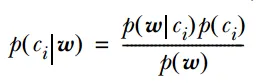
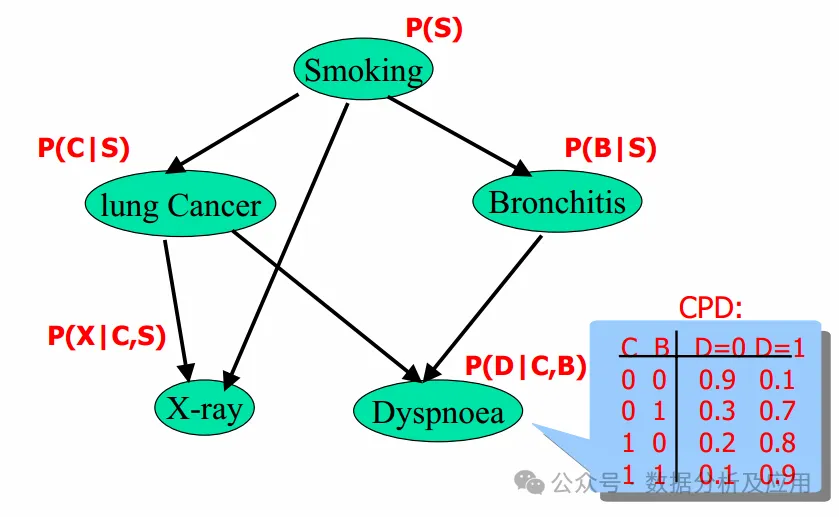
The main representative models include: Naive Bayes classifier, Bayesian networks, and Hidden Markov models. Among them, Naive Bayes classifier and logistic regression are both based on Bayes’ theorem, using probability to express the uncertainty of classification.
Hidden Markov models and Bayesian networks are both probabilistic models used to describe the relationships between random sequences and random variables.
Naive Bayes classifiers and Bayesian networks are both probabilistic graphical models used to describe the probabilistic relationships between random variables.
The following is a code example using the Naive Bayes classifier implemented in Python’s Scikit-learn library:
from sklearn.datasets import load_iris  from sklearn.model_selection import train_test_split  from sklearn.naive_bayes import GaussianNB
# Load dataset  iris = load_iris()  X = iris.data  y = iris.target
# Split into training and testing sets  X_train, X_test, y_train, y_test = train_test_split(X, y, test_size=0.2, random_state=42)
# Build Naive Bayes classifier model  clf = GaussianNB()  clf.fit(X_train, y_train)
# Predict results for test set  y_pred = clf.predict(X_test)
5. Nearest Neighbor Models
Nearest neighbor models (originally intended to be called distance models, but the definition of distance models is broader) are a non-parametric classification and regression method that learns from instances without requiring explicit training and testing set divisions. They determine the similarity of data by measuring the distances between different data points.
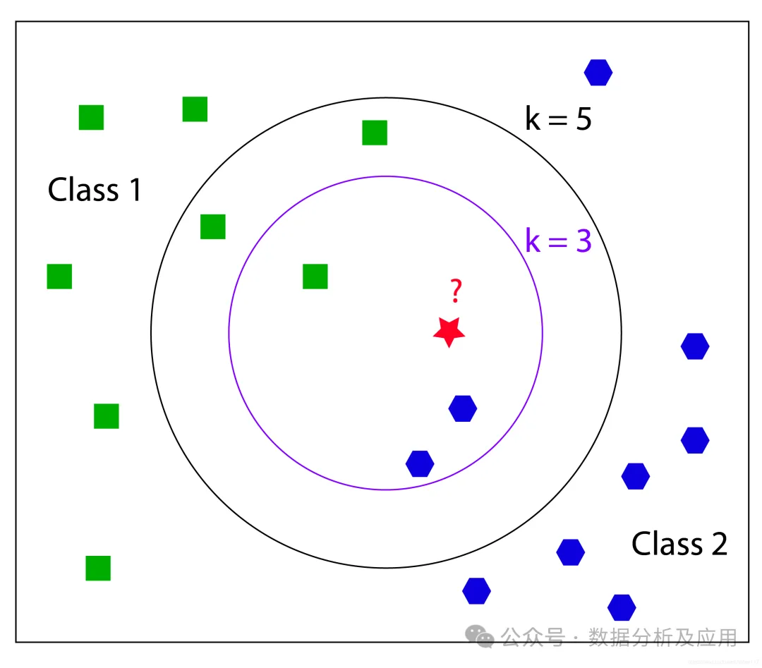
Taking the KNN algorithm as an example, its core idea is that if a sample belongs to the same category as the majority of its k nearest training samples in the feature space, then that sample also belongs to this category. The KNN algorithm learns from instances without requiring explicit training and testing set divisions, determining the similarity of data by measuring the distances between different data points.
Representative models include: k-nearest neighbors algorithm (KNN), radius search, K-means, weighted KNN, multi-level classification KNN, and approximate nearest neighbor (ANN)
The nearest neighbor model is based on similar principles, that is, determining the similarity of data by measuring the distances between different data points.
In addition to the basic KNN algorithm, other variants such as weighted KNN and multi-level classification KNN have improved upon the basic algorithm to better adapt to different classification problems.
Approximate nearest neighbor (ANN) is a method that sacrifices precision for time and space efficiency to find the nearest neighbors from a large sample. The ANN algorithm processes large datasets by reducing storage space and improving lookup efficiency. It reduces search time through an “approximate” method, allowing for a small margin of error during the search.
The following is a code example using the KNN algorithm implemented in Python’s Scikit-learn library:
from sklearn.datasets import load_iris  from sklearn.model_selection import train_test_split  from sklearn.neighbors import KNeighborsClassifier
# Load dataset  iris = load_iris()  X = iris.data  y = iris.target
# Split into training and testing sets  X_train, X_test, y_train, y_test = train_test_split(X, y, test_size=0.2, random_state=42)
# Build KNN classifier model  knn = KNeighborsClassifier(n_neighbors=3)  knn.fit(X_train, y_train)
# Predict results for test set  y_pred = knn.predict(X_test)
6. Ensemble Learning Models
Ensemble Learning is not just a type of model, but a concept of integrating multiple models, combining the prediction results of multiple learners to improve overall prediction accuracy and stability.In practical applications, ensemble learning is undoubtedly a powerful tool for data mining!
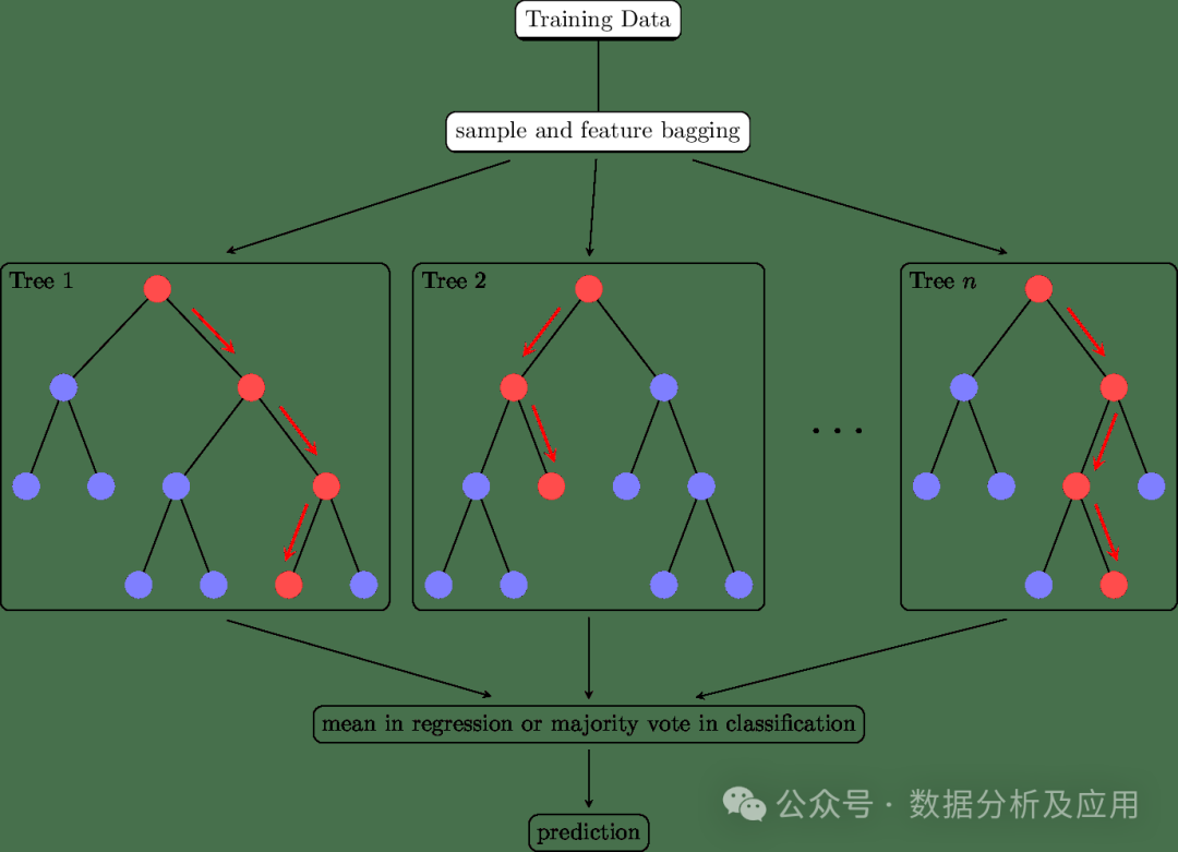
The core idea of ensemble learning is to improve overall predictive performance by integrating multiple base learners. Specifically, by combining the prediction results of multiple learners, we can reduce the overfitting and underfitting problems of a single learner and improve the model’s generalization ability. Additionally, by introducing diversity (such as different base learners, different training data, etc.), the model’s performance can be further improved. Common ensemble learning methods include:
-
Bagging is an ensemble learning method that improves model stability and generalization ability by introducing diversity and reducing variance. It can be applied to any classification or regression algorithm.
-
Boosting is an ensemble learning method that improves model performance by introducing diversity and altering the importance of base learners. It is also a general technique that can be applied to any classification or regression algorithm.
-
Stacking is a more advanced ensemble learning method that combines different base learners into a hierarchical structure and integrates them through a meta-learner. Stacking can be used for classification or regression problems and is typically used to enhance the model’s generalization ability.
Representative models of ensemble learning include: Random Forest, Isolation Forest, GBDT, AdaBoost, Xgboost, etc. The following is a code example using the Random Forest algorithm implemented in Python’s Scikit-learn library:
from sklearn.ensemble import RandomForestClassifier  from sklearn.datasets import load_iris  from sklearn.model_selection import train_test_split
# Load dataset  iris = load_iris()  X = iris.data  y = iris.target
# Split into training and testing sets  X_train, X_test, y_train, y_test = train_test_split(X, y, test_size=0.2, random_state=42)
# Build Random Forest classifier model  clf = RandomForestClassifier(n_estimators=100, random_state=42)  clf.fit(X_train, y_train)
# Predict results for test set  y_pred = clf.predict(X_test)
In summary, by categorizing models with similar principles into various categories, we can explore their principles one by one in a more systematic and comprehensive manner. I hope this is helpful to everyone!