Author Information: First-year graduate student in Computer Science at Xiamen University, welcome everyone to follow my GitHub: xmu-xiaoma666, Zhihu: Work Harder.
In recent years, Attention-based methods have gained popularity in academia and industry due to their interpretability and effectiveness. However, the network structures proposed in papers are often embedded into frameworks for classification, detection, segmentation, etc., leading to redundant code, making it difficult for beginners like me to find the core code of the network, resulting in certain difficulties in understanding the papers and network concepts. Therefore, I have organized and reproduced the core code from the recent papers on Attention, MLP, and Re-parameterization to facilitate readers’ understanding.
This article mainly provides a brief introduction to the Attention part of this project. The project will continue to update the latest paper works. Everyone is welcome to follow and star this work. If there are any issues during the reproduction and organization process, feel free to raise them in the issues section, and I will respond promptly~
Project Address
https://github.com/xmu-xiaoma666/External-Attention-pytorch
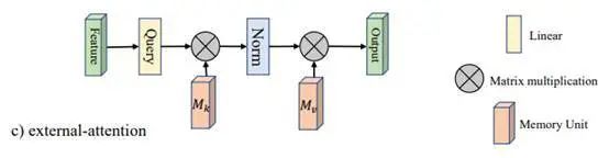
1. External Attention
1.1. Citation
Beyond Self-attention: External Attention using Two Linear Layers for Visual Tasks.—arXiv 2021.05.05
Paper Address: https://arxiv.org/abs/2105.02358
1.2. Model Structure
1.3. Introduction
This is an article published in May on arXiv, mainly addressing two pain points of Self-Attention (SA): (1) O(n^2) computational complexity; (2) SA calculates Attention based on different positions on the same sample, ignoring the relationship between different samples. Therefore, this paper adopts two concatenated MLP structures as memory units, reducing the computational complexity to O(n); additionally, these two memory units learn based on all training data, implicitly considering the relationship between different samples.
1.4. Usage Method
from attention.ExternalAttention import ExternalAttention
import torch

input=torch.randn(50,49,512)
ea = ExternalAttention(d_model=512,S=8)
output=ea(input)
print(output.shape)
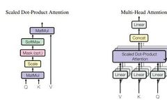
2. Self Attention
2.1. Citation
Attention Is All You Need—NeurIPS2017
Paper Address: https://arxiv.org/abs/1706.03762
2.2. Model Structure
2.3. Introduction
This is an article published by Google in NeurIPS2017, which has had a significant impact in various fields such as CV, NLP, and multimodal processing, with over 22,000 citations. The Self-Attention proposed in the Transformer is a type of Attention used to calculate the weights between different positions in features, thereby updating the features. First, the input feature is mapped through FC to obtain three features: Q, K, and V. Then, the attention map is obtained by multiplying Q and K, and the weighted features are obtained by multiplying the attention map with V. Finally, the features are mapped again through FC to obtain a new feature. (There are many excellent explanations online about Transformers and Self-Attention, so I will not go into detail here.)
2.4. Usage Method
from attention.SelfAttention import ScaledDotProductAttention
import torch
input=torch.randn(50,49,512)
sa = ScaledDotProductAttention(d_model=512, d_k=512, d_v=512, h=8)
output=sa(input,input,input)
print(output.shape)
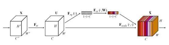
3. Squeeze-and-Excitation (SE) Attention
3.1. Citation
Squeeze-and-Excitation Networks—CVPR2018
Paper Address: https://arxiv.org/abs/1709.01507
3.2. Model Structure
3.3. Introduction
This is a paper from CVPR2018, which is also very influential, with over 7,000 citations. This paper deals with channel attention, and due to its simple structure and effectiveness, it has sparked a wave of interest in channel attention. The idea of this paper is quite simple: first, perform AdaptiveAvgPool on the spatial dimension, then learn channel attention through two FC layers, and normalize with Sigmoid to obtain the Channel Attention Map, which is then multiplied by the original features to obtain the weighted features.
3.4. Usage Method
from attention.SEAttention import SEAttention
import torch
input=torch.randn(50,512,7,7)
se = SEAttention(channel=512,reduction=8)
output=se(input)
print(output.shape)
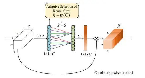
4. Selective Kernel (SK) Attention
4.1. Citation
Selective Kernel Networks—CVPR2019
Paper Address: https://arxiv.org/pdf/1903.06586.pdf
4.2. Model Structure
4.3. Introduction
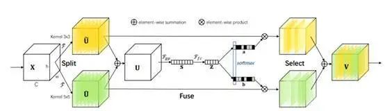
This is a paper from CVPR2019, paying homage to the ideas of SENet. In traditional CNNs, each convolutional layer uses the same size convolution kernel, which limits the model’s expressive ability; whereas the Inception model structure, which is “wider,” has verified that learning with multiple different convolution kernels can indeed enhance the model’s expressive ability. The authors borrowed the idea from SENet, dynamically calculating the weights of each convolution kernel to fuse the results from different convolution kernels.
I believe that the reason this paper can also be called lightweight is that when performing channel attention on different kernels, the parameters are shared (i.e., because before doing Attention, the features are fused, so the results of different convolution kernels share the parameters of one SE module).
This method is divided into three parts: Split, Fuse, Select. Split is a multi-branch operation that convolves using different convolution kernels to obtain different features; the Fuse part uses the SE structure to obtain the channel attention matrix (N convolution kernels can yield N attention matrices, and this operation shares parameters for all features), thus obtaining features after SE from different kernels; the Select operation adds these features together.
4.4. Usage Method
from attention.SKAttention import SKAttention
import torch
input=torch.randn(50,512,7,7)
se = SKAttention(channel=512,reduction=8)
output=se(input)
print(output.shape)
5. CBAM Attention
5.1. Citation
CBAM: Convolutional Block Attention Module—ECCV2018
https://openaccess.thecvf.com/content_ECCV_2018/papers/Sanghyun_Woo_Convolutional_Block_Attention_ECCV_2018_paper.pdf
5.2. Model Structure
5.3. Introduction
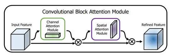
This is a paper from ECCV2018, which simultaneously uses Channel Attention and Spatial Attention, linking the two (the paper also conducted ablation experiments on parallel and two types of serial connections).
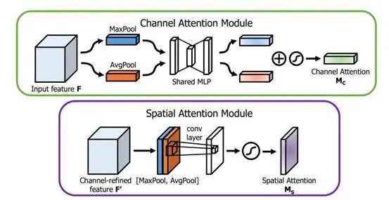
In terms of Channel Attention, the general structure is similar to SE, but the authors propose that AvgPool and MaxPool have different representation effects. Therefore, the authors performed AvgPool and MaxPool on the original features in the Spatial dimension, then extracted channel attention using the SE structure, noting that parameters are shared here, and after adding the two features together, normalization is performed to obtain the attention matrix.
Spatial Attention is similar to Channel Attention; first, pooling is performed in the channel dimension using two types of pooling, then the two features are concatenated, and a 7×7 convolution is used to extract Spatial Attention (the reason for using 7×7 is that the attention extracted is spatial, thus the convolution kernel must be large enough). Finally, normalization is performed to obtain the spatial attention matrix.
5.4. Usage Method
from attention.CBAM import CBAMBlock
import torch
input=torch.randn(50,512,7,7)
kernel_size=input.shape[2]
cbam = CBAMBlock(channel=512,reduction=16,kernel_size=kernel_size)
output=cbam(input)
print(output.shape)
6. BAM Attention
6.1. Citation
BAM: Bottleneck Attention Module—BMCV2018
Paper Address: https://arxiv.org/pdf/1807.06514.pdf
6.2. Model Structure
6.3. Introduction
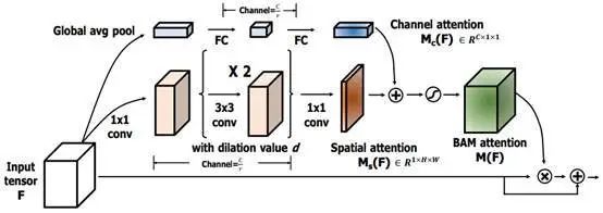
This is a work from the same authors as CBAM, similar in nature, also featuring dual Attention. The difference is that while CBAM concatenates the results of two attentions, BAM directly adds the two attention matrices together.
In terms of Channel Attention, it is basically the same as SE’s structure. For Spatial Attention, pooling is performed in the channel dimension, followed by two 3×3 dilated convolutions, and finally, a 1×1 convolution is used to obtain the Spatial Attention matrix.
Finally, the Channel Attention and Spatial Attention matrices are added together (using broadcasting), and normalization is performed, resulting in a combined attention matrix of spatial and channel attention.
6.4. Usage Method
from attention.BAM import BAMBlock
import torch
input=torch.randn(50,512,7,7)
bam = BAMBlock(channel=512,reduction=16,dia_val=2)
output=bam(input)
print(output.shape)
7. ECA Attention
7.1. Citation
ECA-Net: Efficient Channel Attention for Deep Convolutional Neural Networks—CVPR2020
Paper Address: https://arxiv.org/pdf/1910.03151.pdf
7.2. Model Structure
7.3. Introduction
This is a paper from CVPR2020.
As shown in the figure, SE implements channel attention using two fully connected layers, while ECA requires one convolution. The author’s reasoning is that calculating attention between all channels is unnecessary, and using two fully connected layers indeed introduces too many parameters and computational load.
Therefore, after performing AvgPool, only a one-dimensional convolution with a receptive field of k is used (equivalent to calculating attention only for adjacent k channels), greatly reducing the parameters and computational load (i.e., SE is a global attention, while ECA is a local attention).
7.4. Usage Method
from attention.ECAAttention import ECAAttention
import torch
input=torch.randn(50,512,7,7)
eca = ECAAttention(kernel_size=3)
output=eca(input)
print(output.shape)
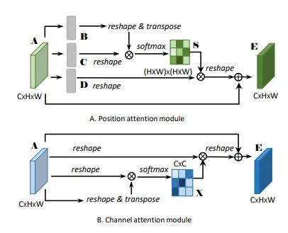
8. DANet Attention
8.1. Citation
Dual Attention Network for Scene Segmentation—CVPR2019
Paper Address: https://arxiv.org/pdf/1809.02983.pdf
8.2. Model Structure
8.3. Introduction
This is an article from CVPR2019, with a very simple idea: applying self-attention to scene segmentation tasks. The difference is that self-attention focuses on the attention between each position, while this paper extends self-attention and adds a channel attention branch, operating similarly to self-attention, but the three Linear layers for generating Q, K, and V are removed. Finally, the features after both attentions are summed element-wise.
8.4. Usage Method
from attention.DANet import DAModule
import torch
input=torch.randn(50,512,7,7)
danet=DAModule(d_model=512,kernel_size=3,H=7,W=7)
print(danet(input).shape)
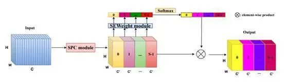
9. Pyramid Split Attention (PSA)
9.1. Citation
EPSANet: An Efficient Pyramid Split Attention Block on Convolutional Neural Network—arXiv 2021.05.30
Paper Address: https://arxiv.org/pdf/2105.14447.pdf
9.2. Model Structure
9.3. Introduction
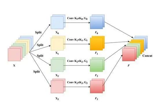
This is an article uploaded on arXiv on May 30 by Shenzhen University, aiming to explore how to acquire and explore spatial information at different scales to enrich the feature space. The network structure is relatively simple, mainly divided into four steps: First, the original features are divided into n groups based on channels, and different scales of convolution are performed on different groups to obtain new features W1; Second, SE is performed on the original features to obtain different attention maps; Third, different groups are subjected to SOFTMAX; Fourth, the obtained attention is multiplied with the original features W1.
9.4. Usage Method
from attention.PSA import PSA
import torch
input=torch.randn(50,512,7,7)
psa = PSA(channel=512,reduction=8)
output=psa(input)
print(output.shape)
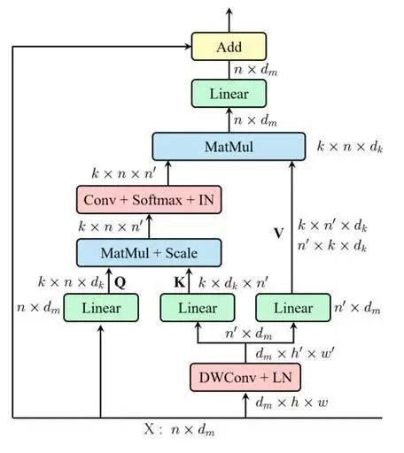
10. Efficient Multi-Head Self-Attention (EMSA)
10.1. Citation
ResT: An Efficient Transformer for Visual Recognition—arXiv 2021.05.28
Paper Address: https://arxiv.org/abs/2105.13677
10.2. Model Structure
10.3. Introduction
This is an article uploaded on May 28 by Nanjing University on arXiv. The main problems addressed are two pain points of SA: (1) The computational complexity of Self-Attention is quadratic in relation to n (where n is the size of the spatial dimension); (2) Each head only has partial information of q, k, v, leading to performance loss if their dimensions are too small. The approach proposed in this paper is quite simple: before the FC in SA, a convolution is used to reduce the spatial dimension, obtaining K and V with smaller spatial dimensions.
10.4. Usage Method
from attention.EMSA import EMSA
import torch
from torch import nn
from torch.nn import functional as F
input=torch.randn(50,64,512)
emsa = EMSA(d_model=512, d_k=512, d_v=512, h=8,H=8,W=8,ratio=2,apply_transform=True)
output=emsa(input,input,input)
print(output.shape)
Conclusion
Currently, the Attention works organized in this project are indeed not comprehensive enough. As the readership increases, this project will be continuously improved. Everyone is welcome to star and support. If there are any inappropriate expressions or mistakes in the code implementation in the article, please feel free to point them out~