
Click on the above “Beginner’s Guide to Vision” to select Star or “Pin”
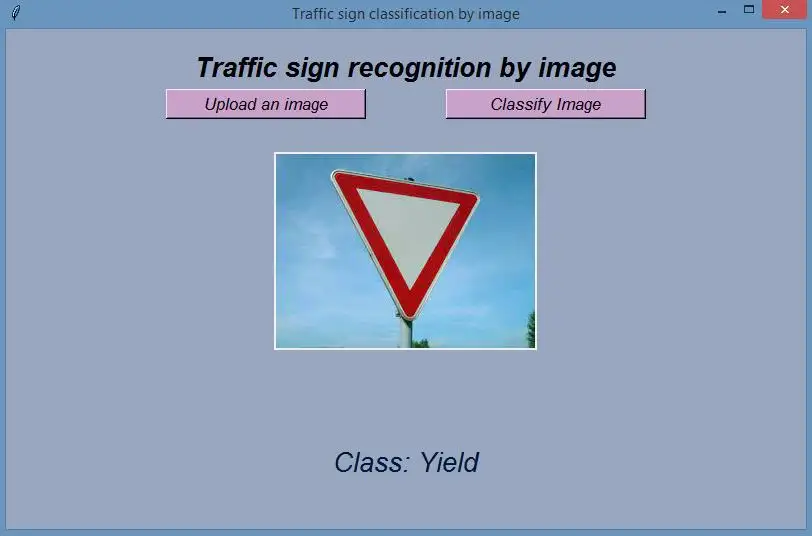
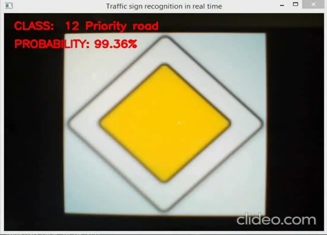
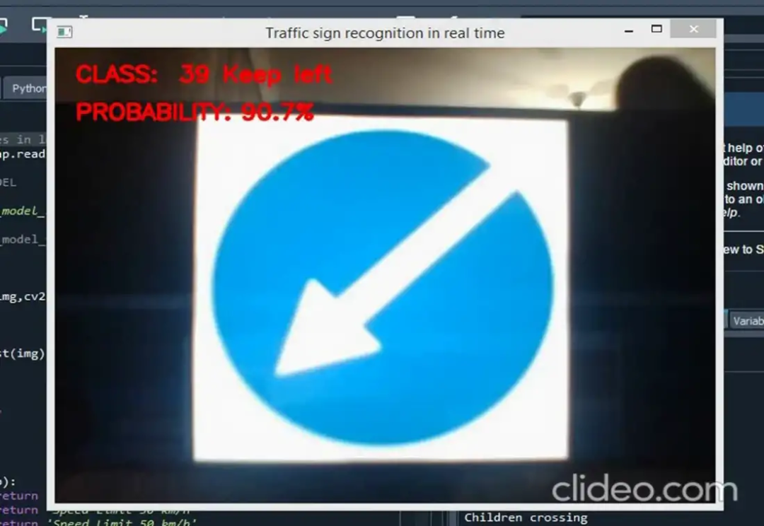
Essential content delivered promptlyIn this article, we establish a CNN model using the Python programming language and libraries Keras and OpenCV, successfully classifying traffic signs with an accuracy of 96%. We developed a traffic sign recognition application that can operate in two modes: image recognition and real-time recognition via a webcam.
GitHub for this article: https://github.com/Daulettulegenov/TSR_CNN
We provide an open-source dataset of traffic signs, hoping it will assist everyone: http://www.nlpr.ia.ac.cn/pal/trafficdata/recognition.html
In recent years, computer vision has been a direction in modern technological development. The primary task of this direction is to classify objects in photos or from cameras. Typically, case-based machine learning methods are used to solve common problems. This article discusses the application of machine learning algorithms in computer vision for traffic sign recognition. Traffic signs are flat man-made objects with fixed shapes. Traffic sign recognition algorithms are applied to two practical problems. The first task is to control autonomous vehicles. A key component of the autonomous vehicle control system is object recognition. The objects recognized are mainly pedestrians, other vehicles, traffic lights, and traffic signs. The second task using traffic sign recognition is to automatically map data based on DVRs installed in cars. Next, we will detail how to build a CNN network capable of recognizing traffic signs.
Import Necessary Libraries
# data analysis and wrangling
import numpy as np
import pandas as pd
import os
import random

# visualization
import matplotlib.pyplot as plt
from PIL import Image

# machine learning
from keras.models import Sequential
from keras.layers import Dense
from tensorflow.keras.optimizers import Adam
from keras.utils.np_utils import to_categorical
from keras.layers import Dropout, Flatten
from keras.layers.convolutional import Conv2D, MaxPooling2D
import cv2
from sklearn.model_selection import train_test_split
from keras.preprocessing.image import ImageDataGenerator
Load Data
The Python Pandas package helps us handle the dataset. We first import the training and testing datasets into Pandas DataFrames. We also combine these datasets to run certain operations together on both datasets.
# Importing of the Images
count = 0
images = []
classNo = []
myList = os.listdir(path)
print("Total Classes Detected:",len(myList))
noOfClasses=len(myList)
print("Importing Classes.....")
for x in range (0,len(myList)):
    myPicList = os.listdir(path+"/"+str(count))
    for y in myPicList:
        curImg = cv2.imread(path+"/"+str(count)+"/"+y)
        curImg = cv2.resize(curImg, (30, 30))
        images.append(curImg)
        classNo.append(count)
    print(count, end =" ")
    count +=1
print(" ")
images = np.array(images)
classNo = np.array(classNo)
To properly train and evaluate the implemented system, we will split the dataset into three groups. Dataset split: 20% test set, 20% validation dataset, and the remaining data used as training dataset.
# Split Data
X_train, X_test, y_train, y_test = train_test_split(images, classNo, test_size=testRatio)
X_train, X_validation, y_train, y_validation = train_test_split(X_train, y_train, test_size=validationRatio)
The dataset contains 34,799 images, consisting of 43 types of traffic signs. These include basic road signs such as speed limit, stop signs, yield, priority road, “no entry”, “pedestrian”, etc.
# DISPLAY SOME SAMPLES IMAGES OF ALL THE CLASSES
num_of_samples = []
cols = 5
num_classes = noOfClasses
fig, axs = plt.subplots(nrows=num_classes, ncols=cols, figsize=(5, 300))
fig.tight_layout()
for i in range(cols):
    for j,row in data.iterrows():
        x_selected = X_train[y_train == j]
        axs[j][i].imshow(x_selected[random.randint(0, len(x_selected)- 1), :, :], cmap=plt.get_cmap("gray"))
        axs[j][i].axis("off")
        if i == 2:
            axs[j][i].set_title(str(j)+ "-"+row["Name"])
            num_of_samples.append(len(x_selected))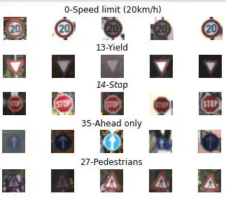
# DISPLAY A BAR CHART SHOWING NO OF SAMPLES FOR EACH CATEGORY
print(num_of_samples)
plt.figure(figsize=(12, 4))
plt.bar(range(0, num_classes), num_of_samples)
plt.title("Distribution of the training dataset")
plt.xlabel("Class number")
plt.ylabel("Number of images")
plt.show()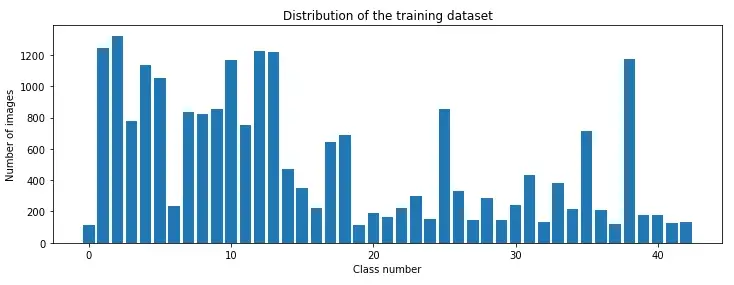
There is a significant imbalance between the classes in the dataset. Some classes have fewer than 200 images, while others have over 1000 images. This means our model may be biased towards overrepresented classes, especially when it is not confident in its predictions. To address this issue, we utilized existing image transformation techniques.
For better classification, all images in the dataset are converted to grayscale images.
# PREPROCESSING THE IMAGES
def grayscale(img):
    img = cv2.cvtColor(img,cv2.COLOR_BGR2GRAY)
    return img

def equalize(img):
    img =cv2.equalizeHist(img)
    return img

def preprocessing(img):
    img = grayscale(img)     # CONVERT TO GRAYSCALE
    img = equalize(img)      # STANDARDIZE THE LIGHTING IN AN IMAGE
    img = img/255            # TO NORMALIZE VALUES BETWEEN 0 AND 1 INSTEAD OF 0 TO 255
    return img

X_train=np.array(list(map(preprocessing,X_train)))  # TO ITERATE AND PREPROCESS ALL IMAGES
X_validation=np.array(list(map(preprocessing,X_validation)))
X_test=np.array(list(map(preprocessing,X_test)))
Data augmentation is a method of enhancing the original dataset. The more data, the higher the results; this is a fundamental rule of machine learning.
#AUGMENTATION OF IMAGES: TO MAKE IT MORE GENERIC
dataGen= ImageDataGenerator(width_shift_range=0.1,   # 0.1 = 10%     IF MORE THAN 1 E.G 10 THEN IT REFERS TO NO. OF  PIXELS E.G 10 PIXELS
                            height_shift_range=0.1,
                            zoom_range=0.2,  # 0.2 MEANS CAN GO FROM 0.8 TO 1.2
                            shear_range=0.1,  # MAGNITUDE OF SHEAR ANGLE
                            rotation_range=10)  # DEGREES
dataGen.fit(X_train)
batches= dataGen.flow(X_train,y_train,batch_size=20)  # REQUESTING DATA GENERATOR TO GENERATE IMAGES  BATCH SIZE = NO. OF IMAGES CREATED EACH TIME IT'S CALLED
X_batch,y_batch = next(batches)
One-hot encoding is used for our categorical values y_train, y_test, y_validation.
y_train = to_categorical(y_train,noOfClasses)
y_validation = to_categorical(y_validation,noOfClasses)
y_test = to_categorical(y_test,noOfClasses)
We create a neural network using the Keras library. Below is the code for creating the model structure:
def myModel():
    model = Sequential()
    model.add(Conv2D(filters=32, kernel_size=(5,5), activation='relu', input_shape=X_train.shape[1:]))
    model.add(Conv2D(filters=32, kernel_size=(5,5), activation='relu'))
    model.add(MaxPooling2D(pool_size=(2, 2)))
    model.add(Dropout(rate=0.25))
    model.add(Conv2D(filters=64, kernel_size=(3, 3), activation='relu'))
    model.add(Conv2D(filters=64, kernel_size=(3, 3), activation='relu'))
    model.add(MaxPooling2D(pool_size=(2, 2)))
    model.add(Dropout(rate=0.25))
    model.add(Flatten())
    model.add(Dense(256, activation='relu'))
    model.add(Dropout(rate=0.5))
    model.add(Dense(43, activation='softmax'))
    model.compile(loss='categorical_crossentropy', optimizer='adam', metrics=['accuracy'])
    return model
# TRAIN
model = myModel()
print(model.summary())
history = model.fit(X_train, y_train, batch_size=batch_size_val, epochs=epochs_val, validation_data=(X_validation,y_validation))The above code uses 6 convolutional layers and 1 fully connected layer. First, we add a convolutional layer with 32 filters to the model. Next, we add a convolutional layer with 64 filters. After each layer, we add a max pooling layer with a window size of 2 × 2. Dropout layers with rates of 0.25 and 0.5 are also added to prevent the network from overfitting. In the last few lines, we add a dense layer that performs classification among 43 classes using the softmax activation function.
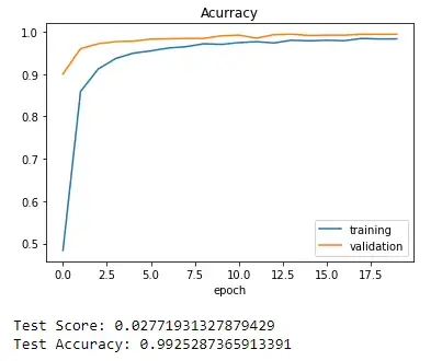
At the end of the last epoch, we obtained the following values: loss = 0.0523; accuracy = 0.9832; Val_loss = 0.0200; Val_accuracy = 0.9943; this result looks very good. Afterward, we plot our training process.
#PLOT
plt.figure(1)
plt.plot(history.history['loss'])
plt.plot(history.history['val_loss'])
plt.legend(['training','validation'])
plt.title('loss')
plt.xlabel('epoch')
plt.figure(2)
plt.plot(history.history['accuracy'])
plt.plot(history.history['val_accuracy'])
plt.legend(['training','validation'])
plt.title('Accuracy')
plt.xlabel('epoch')
plt.show()
score =model.evaluate(X_test,y_test,verbose=0)
print('Test Score:',score[0])
print('Test Accuracy:',score[1])
#testing accuracy on test dataset
from sklearn.metrics import accuracy_score

y_test = pd.read_csv('Test.csv')
labels = y_test["ClassId"].values
imgs = y_test["Path"].values
data=[]
for img in imgs:
    image = Image.open(img)
    image = image.resize((30,30))
    data.append(np.array(image))
X_test=np.array(data)
X_test=np.array(list(map(preprocessing,X_test)))
predict_x=model.predict(X_test)
pred=np.argmax(predict_x,axis=1)
print(accuracy_score(labels, pred))
We tested the constructed model on the test dataset and achieved 96% accuracy.
Using the built-in function model_name.save(), we can save a model for future use. This function saves the model in a local .p file, so we don’t have to retrain the model repeatedly, wasting a lot of time.
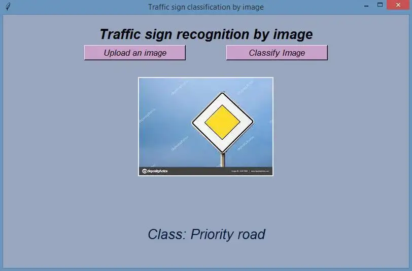
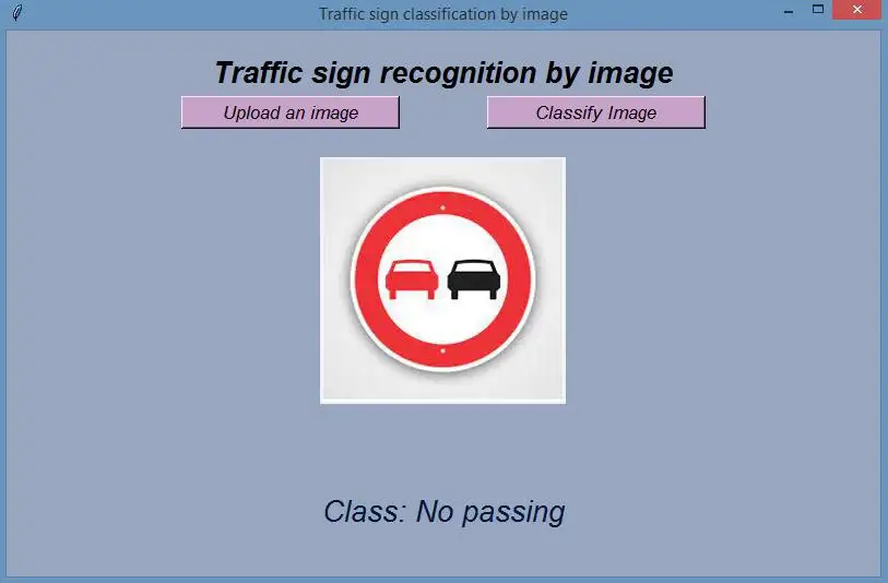
model.save("CNN_model_3.h5")Next, let’s look at some recognition results.
Good news!<br/>Beginner's Guide to Vision knowledge circle is now open to the public👇👇👇<br/><br/>Download 1: OpenCV-Contrib Extension Module Chinese Tutorial<br/>Reply in the "Beginner's Guide to Vision" WeChat public account: Extension Module Chinese Tutorial to download the first Chinese version of the OpenCV extension module tutorial available online, covering over twenty chapters including extension module installation, SFM algorithms, stereo vision, target tracking, biological vision, super-resolution processing, etc.<br/><br/>Download 2: Python Vision Practical Project 52 Lectures<br/>Reply in the "Beginner's Guide to Vision" WeChat public account: Python Vision Practical Project to download 31 practical vision projects including image segmentation, mask detection, lane line detection, vehicle counting, eyeliner addition, license plate recognition, character recognition, emotion detection, text content extraction, facial recognition, etc., to help you quickly learn computer vision.<br/><br/>Download 3: OpenCV Practical Projects 20 Lectures<br/>Reply in the "Beginner's Guide to Vision" WeChat public account: OpenCV Practical Projects 20 Lectures to download 20 practical projects based on OpenCV, achieving advanced learning in OpenCV.<br/><br/>Discussion Group<br/>Welcome to join the reader group of the WeChat public account to communicate with peers. Currently, there are WeChat groups for SLAM, 3D vision, sensors, autonomous driving, computational photography, detection, segmentation, recognition, medical imaging, GAN, algorithm competitions, etc. (will gradually be subdivided in the future). Please scan the WeChat number below to join the group, and note: "Nickname + School/Company + Research Direction", for example: "Zhang San + Shanghai Jiao Tong University + Vision SLAM". Please follow the format for notes; otherwise, you will not be accepted. After successful addition, you will be invited to join relevant WeChat groups based on research direction. Please do not send advertisements in the group; otherwise, you will be removed from the group. Thank you for your understanding~