A Deep Dive into GoogLeNet: Evolution from Inception v1 to v4

In 2014, GoogLeNet and VGG were the two leading models in that year’s ImageNet competition (ILSVRC14), with GoogLeNet taking first place and VGG second. A common feature of these two model architectures is their increased depth. VGG inherits some structural elements from LeNet and AlexNet, while GoogLeNet made bolder structural attempts. Although it has only 22 layers, it is much smaller than both AlexNet and VGG, with GoogLeNet having 5 million parameters compared to AlexNet’s 12 times that and VGG’s 3 times AlexNet’s. Therefore, GoogLeNet is a better choice when memory or computational resources are limited; moreover, from the model results, GoogLeNet’s performance is superior.

Fun Fact: GoogLeNet is a deep network architecture developed by Google. It is named “GoogLeNet” as a tribute to “LeNet” rather than being called “GoogleNet”.

So how does GoogLeNet further enhance performance? Generally, the most direct way to improve network performance is to increase its depth and width, where depth refers to the number of layers and width refers to the number of neurons. However, this method has several issues: (1) Too many parameters can easily lead to overfitting, especially when the training dataset is limited; (2) Larger networks with more parameters increase computational complexity, making them difficult to apply; (3) Deeper networks are prone to the vanishing gradient problem (gradients tend to disappear as they propagate back), making it hard to optimize the model. Thus, some jokingly say that “deep learning” is really just “deep hyperparameter tuning.” The solution to these problems is to increase the network’s depth and width while reducing the number of parameters. To reduce parameters, the idea of converting fully connected layers to sparse connections naturally arises. However, in practice, changing fully connected layers to sparse connections does not significantly reduce computational load because most hardware is optimized for dense matrix calculations. Sparse matrices, while having less data, are often slow to compute.

Is there a method that can maintain the sparsity of the network structure while leveraging the high computational performance of dense matrices? A significant amount of literature suggests that clustering sparse matrices into denser submatrices can improve computational performance. Just as the human brain can be viewed as a repetitive accumulation of neurons, the GoogLeNet team proposed the Inception network structure, which constructs a “base neuron” architecture to build a sparse, high-performance network structure.

The question arises: what is Inception? Inception has undergone several iterations from V1 to V2, V3, and V4, continuously improving along the way. Below, each version will be introduced one by one.

1. Inception V1

Paper link: Going Deeper with Convolutions

Main contribution: Proposed the Inception convolutional network structure.

1.1 Principle

The paper mentions that to achieve a higher recognition rate, it is natural to think of increasing the number of layers (making the network deeper) and the number of convolutions per layer (making the network wider). However, this leads to two problems: first, the parameters become too large, which can easily lead to overfitting, especially when the dataset is limited, and acquiring an effective dataset is very challenging and often requires extensive human labor for labeling; the second drawback is that it can lead to a lot of redundant computations. The solution to this problem is to use a sparser network structure, but current computational devices struggle with unevenly distributed and sparse computations. The Inception structure was proposed to approximate a sparse distribution, with the main idea being to consider how to approximate a locally optimal sparse convolutional visual network structure.

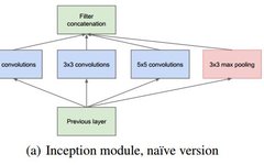
By designing a sparse network structure that can produce dense data, it increases the performance of the neural network while ensuring the efficiency of computational resource usage. Google proposed the basic structure of the original Inception.

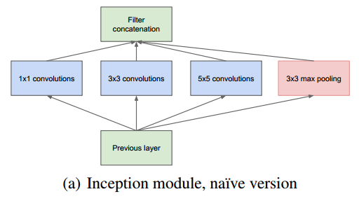
This structure stacks commonly used convolutions (1×1, 3×3, 5×5) and pooling operations (3×3) in CNNs together (the size after convolution and pooling remains the same, and the channels are summed). On one hand, it increases the network’s width, and on the other hand, it enhances the network’s adaptability to scale.

First, looking at the first structure, there are four channels with 1×1, 3×3, and 5×5 convolution kernels. This structure has several characteristics:

1. Using convolution kernels of different sizes means different receptive fields; the final concatenation means the fusion of features at different scales; 2. The choice of 1×1, 3×3, and 5×5 convolution kernel sizes is mainly for alignment convenience. After setting the convolution stride to 1, different-sized convolution kernels can achieve the same dimensional features by setting padding to 0, 1, and 2 respectively, and using same convolution; 3. Many studies indicate that pooling is quite effective, so pooling is also embedded in Inception; 4. As the network progresses, features become more abstract, and the receptive field for each feature also enlarges; with increasing layers, the proportion of 3×3 and 5×5 convolutions should also increase.

The convolutional layers of the network can extract every detail of the input, while the 5×5 filter can cover most of the inputs of the receptive layer. A pooling operation can also be performed to reduce spatial dimensions and decrease overfitting. On top of these layers, a ReLU operation should be performed after each convolutional layer to enhance the network’s non-linear characteristics. However, in the original version of Inception, all convolutional kernels are applied to all outputs from the previous layer, which results in a significant computational load due to the thickness of the feature map. To avoid this, 1×1 convolution kernels are added before the 3×3 and 5×5 convolutions and after max pooling to reduce the thickness of the feature map, thus forming the Inception v1 network structure, as shown in the figure below:

What is the purpose of the 1×1 convolution kernel? The main purpose of the 1×1 convolution is to reduce dimensions and correct linear activation (ReLU). For instance, if the output from the previous layer is 100x100x128, after passing through a 5×5 convolution layer with 256 channels (stride=1, pad=2), the output data is 100x100x256, where the convolution layer’s parameters are 128x5x5x256=819200. However, if the output from the previous layer first passes through a 1×1 convolution layer with 32 channels, and then through a 5×5 convolution layer with 256 outputs, the output data remains 100x100x256, but the number of convolution parameters has been reduced to 128x1x1x32 + 32x5x5x256=204800, approximately a fourfold reduction.

1.2 Network Structure

The GoogLeNet network structure based on Inception is as follows (22 layers in total):

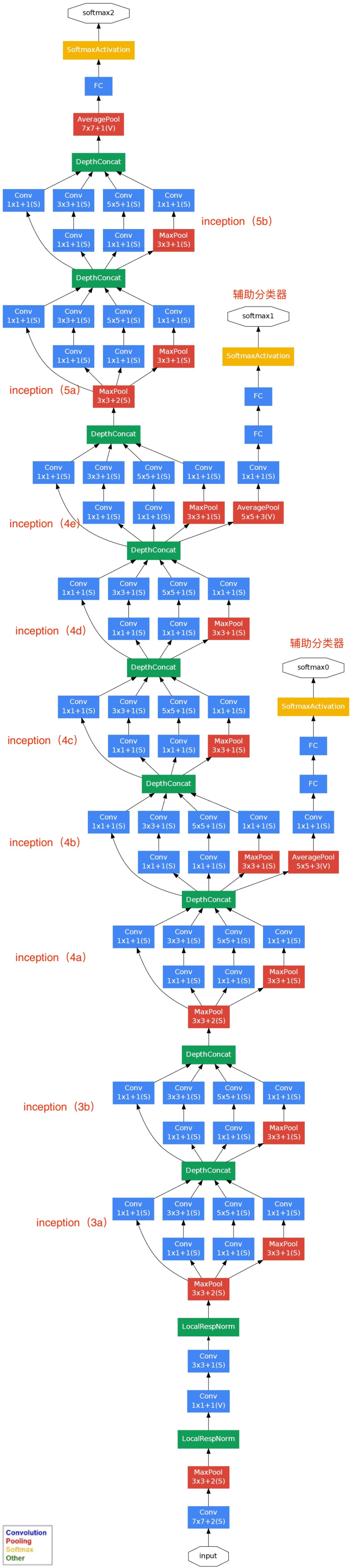
The explanation for the above figure is as follows: (1) GoogLeNet adopts a modular structure of Inception (9 modules), totaling 22 layers, facilitating additions and modifications; (2) The network finally uses average pooling instead of a fully connected layer, a concept derived from NIN (Network in Network), which has been proven to increase accuracy by 0.6%. However, in practice, a fully connected layer is still added at the end for flexibility in output adjustments; (3) Although the fully connected layer has been removed, Dropout is still used in the network; (4) To avoid gradient vanishing, the network adds two auxiliary softmax layers to forward propagate gradients (auxiliary classifiers). The auxiliary classifiers use the output of an intermediate layer for classification and add it to the final classification result with a smaller weight (0.3), effectively performing model blending while providing additional gradient signals for backpropagation, which is beneficial for the training of the entire network. In actual testing, these two additional softmax layers are removed.

The detailed structure diagram of GoogLeNet is as follows:

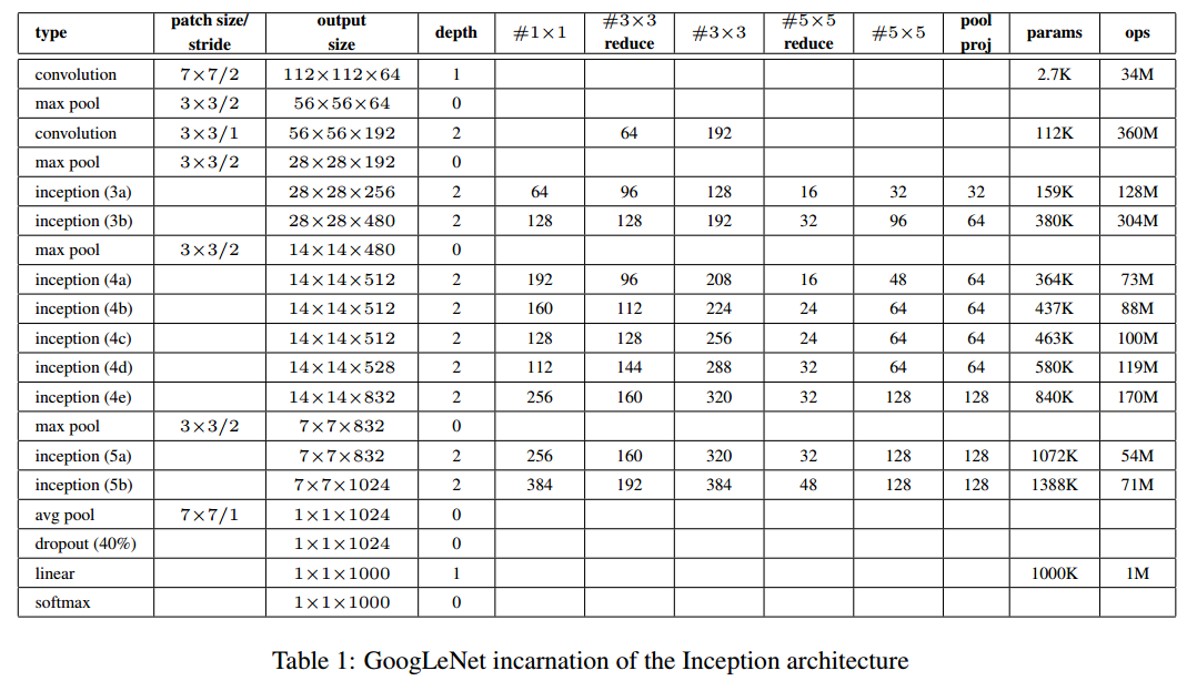
Note: In the table above, “#3×3 reduce” and “#5×5 reduce” indicate the number of 1×1 convolutions used before the 3×3 and 5×5 convolution operations.

The detailed breakdown of the GoogLeNet network structure is as follows:

0. Input The original input image is 224x224x3, and zero-mean normalization preprocessing has been performed (each pixel of the image is subtracted by the mean).

1. First Layer (Convolution Layer) Uses a 7×7 convolution kernel (sliding stride 2, padding 3), 64 channels, outputting 112x112x64, followed by a ReLU operation and a 3×3 max pooling (stride 2), resulting in ((112 – 3 + 1)/2) + 1 = 56, i.e., 56x56x64, followed by another ReLU operation.

2. Second Layer (Convolution Layer) Uses a 3×3 convolution kernel (sliding stride 1, padding 1), 192 channels, outputting 56x56x192, followed by a ReLU operation and a 3×3 max pooling (stride 2), resulting in ((56 – 3 + 1)/2) + 1 = 28, i.e., 28x28x192, followed by another ReLU operation.

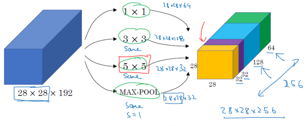
3a. Third Layer (Inception 3a Layer) Divided into four branches, using convolution kernels of different scales:

(1) 64 1×1 convolution kernels, followed by ReLU, outputting 28x28x64; (2) 96 1×1 convolution kernels, used for dimensionality reduction before the 3×3 convolution, transforming into 28x28x96, then ReLU, followed by 128 3×3 convolutions (padding 1), outputting 28x28x128; (3) 16 1×1 convolution kernels, used for dimensionality reduction before the 5×5 convolution, transforming into 28x28x16, followed by ReLU and then 32 5×5 convolutions (padding 2), outputting 28x28x32; (4) Pooling layer, using a 3×3 kernel (padding 1), outputting 28x28x192, followed by 32 1×1 convolutions, outputting 28x28x32. The results of these four branches are concatenated along the third dimension, resulting in 64 + 128 + 32 + 32 = 256, with a final output of 28x28x256.

3b. Third Layer (Inception 3b Layer) (1) 128 1×1 convolution kernels, followed by ReLU, outputting 28x28x128; (2) 128 1×1 convolution kernels, used for dimensionality reduction before the 3×3 convolution, transforming into 28x28x128, followed by ReLU and then 192 3×3 convolutions (padding 1), outputting 28x28x192; (3) 32 1×1 convolution kernels, used for dimensionality reduction before the 5×5 convolution, transforming into 28x28x32, followed by ReLU and then 96 5×5 convolutions (padding 2), outputting 28x28x96; (4) Pooling layer, using a 3×3 kernel (padding 1), outputting 28x28x256, followed by 64 1×1 convolutions, outputting 28x28x64. The results of these four branches are concatenated along the third dimension, resulting in 128 + 192 + 96 + 64 = 480, with a final output of 28x28x480.

Layers 4 (4a, 4b, 4c, 4d, 4e), 5 (5a, 5b)… are similar to 3a and 3b, so I won’t repeat them here.

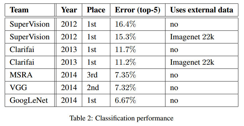
From the experimental results of GoogLeNet, the effect is quite evident, with an error rate lower than that of MSRA, VGG, and other models, as shown in the comparison table below:

1.3 Role of Inception

The authors pointed out the advantages of Inception:

• Significantly increases the number of units at each step, while the computational complexity remains manageable, with larger block convolutions being reduced in dimension first.

• Visual information is processed and aggregated at different scales, allowing features to be extracted from various scales in the next step.

However, specifically why Inception works has remained unclear. The authors later proved the effectiveness of GoogLeNet through experiments, but did not elaborate on the reasons. Deep learning is a field that often prioritizes practice over theory, and its effectiveness is often validated through practical application. Later, I came across a blog that clarified my confusion. The answer provided was:

The role of Inception: to replace the manual determination of filter types in convolution layers or whether to create convolution and pooling layers; that is, there is no need for human decisions regarding which filters to use or whether pooling layers are necessary, as the network can autonomously decide these parameters, allowing it to learn what parameters it needs.

2. Inception V2

Paper link: Rethinking the Inception Architecture for Computer Vision

Inception V2 made the following improvements over Inception V1:

• Introduced Batch Normalization layers, with the standard structure being: convolution-BN-ReLU, reducing Internal Covariate Shift, normalizing each layer’s output to a Gaussian distribution N(0, 1);

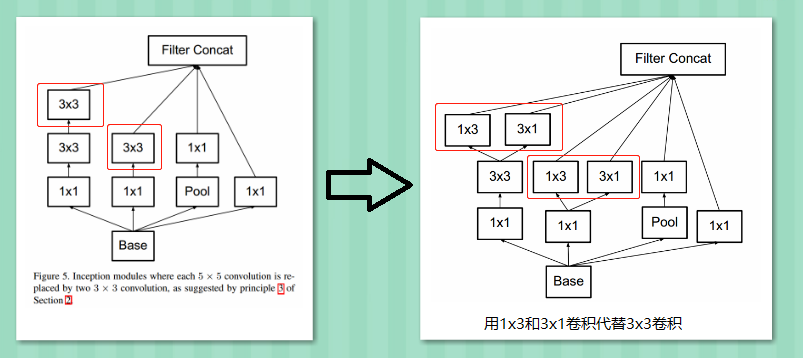
• Decomposed larger convolutions into smaller ones, borrowing from VGG’s approach by using two 3×3 convolutions in series to replace the 5×5 convolution in the Inception module. This is because two 3×3 convolutions have the same receptive field as a single 5×5 convolution but require fewer parameters. Additionally, by adding another layer of convolution, it introduces another ReLU, enhancing the discriminative power of feature information;

• Utilized asymmetric convolutions, further decomposing 3×3 convolutions into 3×1 and 1×3 convolutions;

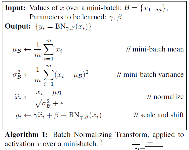
2.1 Batch Normalization

This algorithm is remarkable, making it possible to train deep neural networks.

2.1.1 What Problem Does BN Address?

When training deep neural networks, the authors raised an issue called “Internal Covariate Shift.” This problem arises due to changes in network parameters during the training process. Specifically, for a neural network, the input to the nth layer is the output from the n-1 layer, and as parameters change with each training iteration, the output from the n-1 layer can differ for the same input, leading to variations in the input to the nth layer, which is termed “Internal Covariate Shift.”

2.1.2 Origin of BN

Whitening operation – In traditional machine learning, images are often subjected to a whitening operation before feature extraction, transforming input data into a normal distribution with zero mean and unit variance. The input to convolutional neural networks is images, and whitening can accelerate convergence. In deep networks, each hidden layer’s output serves as the input for the next hidden layer, meaning each hidden layer’s input can undergo a whitening operation. Regularization can be performed on each mini-batch during training:

2.1.3 Essence of BN

My understanding of BN’s main functions is:

• Accelerating network training
• Preventing gradient vanishing

If the activation function is sigmoid, for each neuron, the input distribution gradually approaches the saturation regions of the non-linear mapping, forcing it back to a standard normal distribution with zero mean and unit variance. This ensures the input remains in the active region of the activation function, where the gradient is large, thus accelerating network training and preventing gradient vanishing. Based on this, BN has a significant effect on the sigmoid function. The sigmoid function in the interval [-1, 1] is approximately linear. Without this formula:

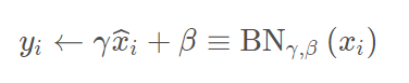
the model’s expressive ability would decrease, making the network approximate a linear mapping. Thus, scale and shift were added. Their primary function is to find a balance between linear and non-linear mappings, allowing for strong non-linear expressive ability while avoiding slow convergence due to non-linear saturation.

2.2 Factorizing Convolutions

2.2.1 Decomposing into Smaller Convolutions

Large convolution kernels can lead to larger receptive fields but also mean more parameters; for instance, a 5×5 kernel has 25 parameters, while a 3×3 kernel has 9 parameters, making the former 2.78 times larger. Thus, the GoogLeNet team borrowed from VGG’s usage to replace a single 5×5 convolution layer with two consecutive 3×3 layers, thereby maintaining the receptive field while reducing the number of parameters, as shown below:

2.2.2 Decomposing into Asymmetric Convolutions

It can be seen that larger convolution kernels can be replaced by a series of 3×3 kernels. But can they be decomposed even further? The GoogLeNet team considered nx1 convolution kernels.

Using asymmetric convolutions, an nxn convolution can be decomposed into a series of 1xn and nx1 convolutions. As shown in the figure, a 3×3 convolution can be decomposed into 3×1 and 1×3 convolutions, saving 33% of the computational load.

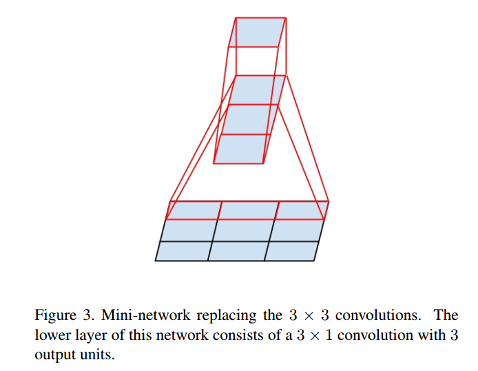
Thus, any nxn convolution can be replaced by a 1xn convolution followed by an nx1 convolution. The GoogLeNet team found that using this decomposition early in the network does not yield good results; it performs better on moderately sized feature maps (suggested size between 12 and 20).

Regarding asymmetric convolutions, the paper mentions:

• The result of first performing an n×1 convolution followed by a 1×n convolution is equivalent to directly performing an n×n convolution.
• Asymmetric convolutions can reduce computational load; originally n×n multiplications are reduced to 2×n multiplications, and the larger n is, the more significant the reduction in operations.
• While this method can lower computational load, it is not universally applicable; asymmetric convolutions should not be used near the input layers as they may affect accuracy; they should be utilized in higher layers, specifically when feature map sizes are between 12×12 and 20×20, where they perform best.

2.3 Reducing Feature Map Size

Generally, if one wants to reduce the image size, there are two methods:

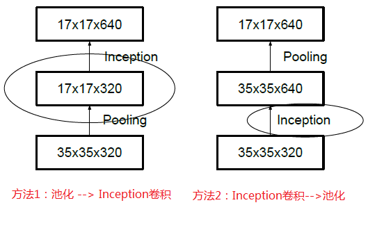
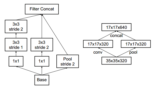
First pooling and then performing Inception convolutions, or performing Inception convolutions followed by pooling. However, method one (left image) leads to bottlenecks in feature representation (loss of features), while method two (right image) is normal but computationally intensive. To maintain feature representation while reducing computational load, the network structure is modified as shown below, using two parallel modules to decrease computational load (convolution and pooling execute in parallel and then merge).

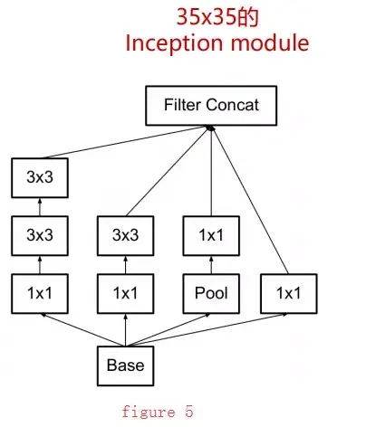
Inception v2 includes the following three different Inception modules:

• The first module (figure 5) is used on 35×35 feature maps, mainly replacing a 5×5 convolution with two 3×3 convolutions.

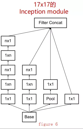
• The second module (figure 6) further decomposes 3×3 convolution kernels into nx1 and 1xn convolutions, used on 17×17 feature maps, with the specific module structure shown below:

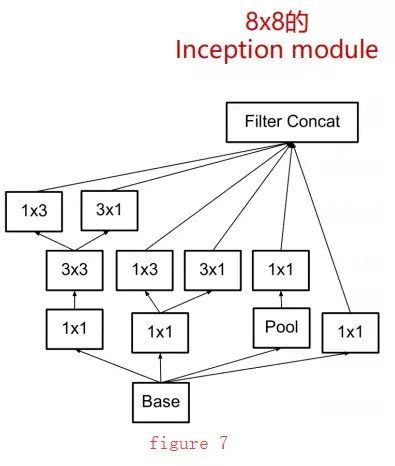
• The third module (figure 7) is mainly used on high-dimensional features, applied to 8×8 feature maps, with the specific structure shown below:

Using Inception V2 to create an improved version of GoogLeNet, the network structure diagram is as follows:

Note: In the table above, Figure 5 refers to the non-evolved Inception, Figure 6 refers to the small convolution version of Inception (using 3×3 kernels instead of 5×5 kernels), and Figure 7 refers to the asymmetric version of Inception (using 1xn and nx1 kernels instead of nxn kernels).

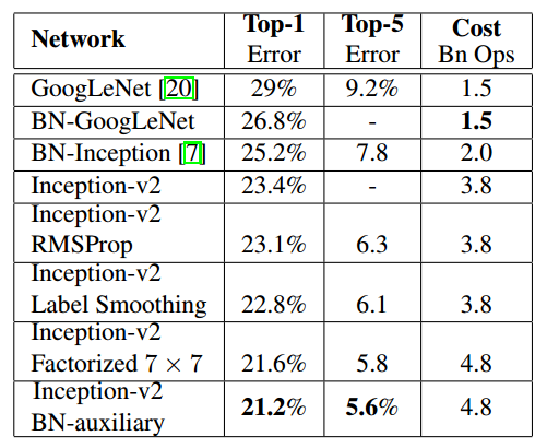
Experiments show that the model results have significantly improved compared to the old GoogLeNet, as shown in the table below:

3. Inception V3

Paper link: Rethinking the Inception Architecture for Computer Vision

Inception v3 overall adopts the network structure of Inception v2, with improvements in optimization algorithms, regularization, and more, specifically:

1. Uses RMSProp as the optimization algorithm instead of SGD.

2. Batch Normalization operations are also added to the auxiliary classifiers.

3. Utilizes Label Smoothing Regularization (LSR) methods to avoid overfitting, preventing the network from being overly confident in predictions for a particular class and increasing attention to low-probability classes. (For more on the LSR optimization method, refer to this blog: https://blog.csdn.net/lqfarmer/article/details/74276680)

4. The most significant improvement is convolution factorization, decomposing 7×7 into two 1D convolutions (1×7, 7×1) and similarly for 3×3 (1×3, 3×1).

5. The network input size changed from 224×224 to 299×299.

4. Inception V4

Paper link: Inception-v4, Inception-ResNet and the Impact of Residual Connections on Learning

The central idea: This paper proposed three networks at once: Inception v4, Inception-ResNet v1, and Inception ResNet v2, primarily because the authors found ResNet effective and decided to combine it with the Inception module to add shortcuts.

Residual connections were introduced to combine Inception and ResNet, making the network both wide and deep, resulting in two versions:

• Inception-ResNet v1: Inception plus ResNet, with computational load comparable to Inception v3, a smaller model.
• Inception-ResNet v2: Inception plus ResNet, with computational load comparable to Inception v4, a larger model, of course with higher accuracy.

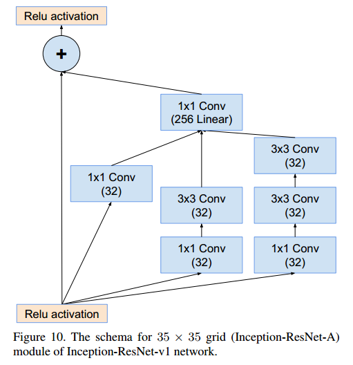
The Inception module of Inception-ResNet-v1 is compared to the original Inception module, increasing the shortcut structure, and a linear 1×1 convolution is used to align dimensions before addition. The Inception-ResNet-v2 model is similar to v1, with different parameter settings.

The Inception-ResNet-v1 Inception module:

1. Inception modules are simplified, not using as many branches, as the identity part (the directly connected line) contains rich feature information;
2. Each Inception module does not use pooling;
3. Each Inception module concludes with a 1×1 convolution (linear activation) to ensure that the identity and Inception parts output features of the same dimension, allowing for their addition.

4.1 Inception v4

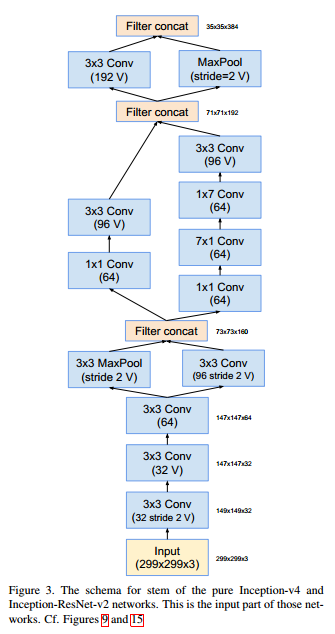
The authors state that due to historical reasons, Inception v3 inherited too many historical burdens, making it look overly complex (yes = =), thus the design was not optimal. The technical limitations were mainly to allow the model to be trained in a distributed manner on DistBelief, which required compromises. Now that it has migrated to TensorFlow (the paper also gives TensorFlow a shout-out), unnecessary historical burdens have been removed to create a simpler and more consistent network design, leading to Inception v4:

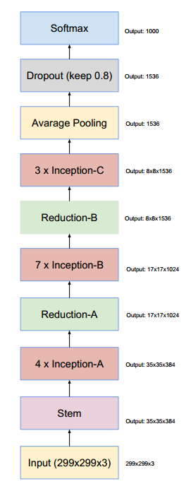
The Stem is the backbone of the Inception-v4 structure, serving the basic feature extraction function. Inception modules are suitable for the intermediate layers of CNNs, processing high-dimensional features. If Inception modules are applied directly to low-dimensional features, the model’s performance will decrease.

Inception-v4 uses four Inception-A modules, seven Inception-B modules, and three Inception-C modules to perform high-level feature extraction. Furthermore, the input and output dimensions of each Inception module are the same, with Inception-A, Inception-B, and Inception-C handling input dimensions of 35×35, 17×17, and 8×8 feature maps, respectively. This design is straightforward, directly indicating which module is most suitable for which size feature map, allowing users to select the appropriate module based on size.

Inception-v4 employs two Reduction modules, Reduction-A and Reduction-B, to reduce the feature map size while increasing its depth without creating bottlenecks. The principle behind the Reduction module is detailed in the paper Rethinking the Inception Architecture for Computer Vision; simply put, it simultaneously reduces size across multiple branches and merges the outputs along the depth dimension.

Inception-v4 uses the average-pooling method from Network in Network to avoid generating a large number of parameters from fully connected layers, reducing the network’s parameter count by 8x8x1536x1536=144M. The final layer uses softmax to obtain the posterior probabilities for each class, with Dropout regularization added to prevent overfitting.

**Note:** In the following text, unless otherwise specified, operations without marked stride=2 and symbol V are assumed to have stride=1 and padding=SAME; if marked with symbol V, padding is assumed to be VALID.

Stem (299x299x3 → 35x35x384)

The 71x71x192 filter concat followed by a 3×3 Conv should be (192 stride=2 V).

Assuming the input image size for the network is 299x299x3, the output after Stem is 35x35x384. To facilitate understanding of the changes in feature map dimensions, the size calculation formula is given: o=⌈(i-k+2p)/2 + 1⌉, where o is the output size, i is the input size, k is the kernel size, and p is the padding.

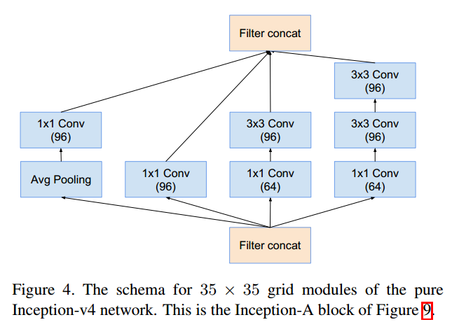
Inception-A (35x35x384 → 35x35x384)

Reduction-A (35x35x384 → 17x17x1024)

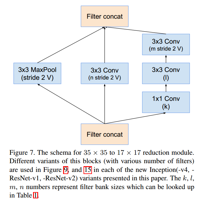
Where k=192, l=224, m=256, n=384.

Inception-B (17x17x1024 → 17x17x1024)

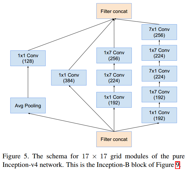
**Question:** The two 1×7 Conv in the third channel may be a typographical error by the author; on GitHub, this part is a 1×7 Conv and a 7×1 Conv.

Reduction-B (17x17x1024 → 8x8x1536)

Inception-C (8x8x1536 → 8x8x1536)

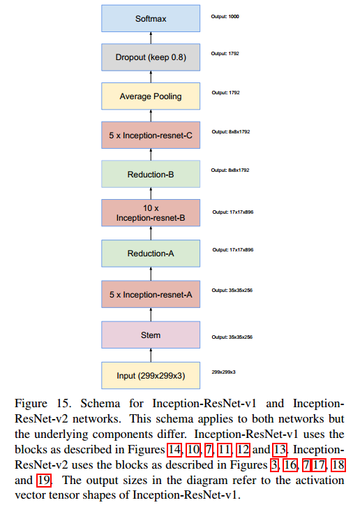
4.2 Inception-ResNet-v1

The Inception-ResNet network introduces the residual structure of ResNet into the Inception module, with two versions: Inception-ResNet-v1 corresponds to Inception-v3, with similar computational complexity, while Inception-ResNet-v2 corresponds to Inception-v4, also with similar computational complexity. The Inception-ResNet network structure is illustrated below:

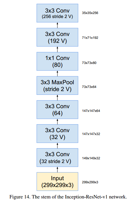
Stem

The structures of the stem modules for Inception-ResNet-v1 and Inception-ResNet-v2 are shown on the right, which are the same as those of Inception-v3 and Inception-v4.

The structure of the Stem module is identical to that of Inception-v3:

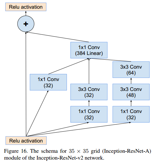
Inception-ResNet-A(35x35x384 → 17x17x1024)

Reduction-A(35x35x384 → 17x17x1024)

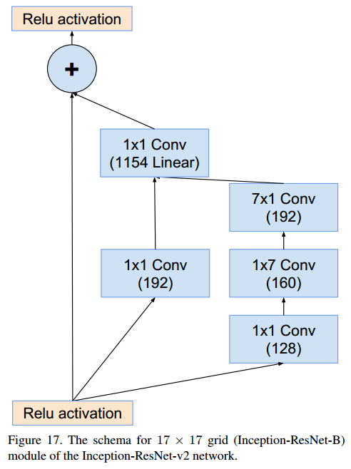
Inception-B (17x17x1024 → 17x17x1024)

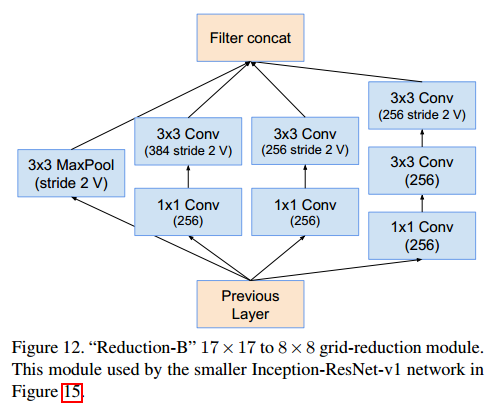
Reduction-B (17x17x1024 → 8x8x1536)

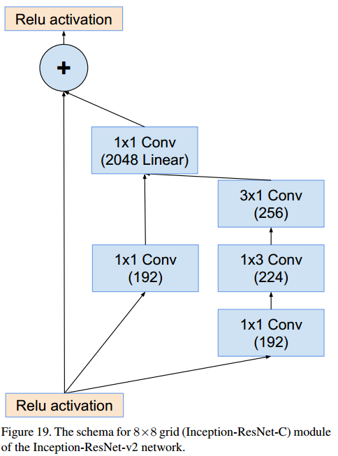
Inception-C (8x8x1536 → 8x8x1536)

4.3 Inception-ResNet-v2

The Inception-ResNet network introduces the residual structure of ResNet into the Inception module, with two versions: Inception-ResNet-v1 corresponds to Inception-v3, while Inception-ResNet-v2 corresponds to Inception-v4. The structure of the Inception-ResNet network is illustrated below:

Stem

The structure of the Stem module is the same as that of Inception-v4:

Inception-ResNet-A(35x35x384 → 17x17x1024)

Reduction-A(35x35x384 → 17x17x1024)

Inception-B (17x17x1024 → 17x17x1024)

Reduction-B (17x17x1024 → 8x8x1536)

Inception-C (8x8x1536 → 8x8x1536)

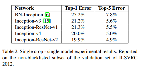
4.4 Performance

The comparison results of different Inception networks on ImageNet are shown in the table below, indicating that the addition of residual structures does not significantly enhance model performance. However, the authors found that residual structures help accelerate convergence. Hence, the authors state that it is still possible to train very deep networks without residual structures.

4.5 Residual Connection

The authors re-examined the role of residual connections, noting that they do not significantly improve model accuracy but accelerate training convergence:

Although the residual version converges faster, the final accuracy seems to mainly depend on the model size.

The authors discovered that if the number of filters exceeds 1000, the residual network becomes unstable, and the network ‘dies’ early in training, meaning that after thousands of iterations, the layers before the average pooling layer only output zeros. Even lowering the learning rate or adding extra BN layers cannot prevent this.

The authors found that scaling the residuals before adding them to the activations of the previous layer can stabilize the training process. Typically, a scaling factor between 0.1 and 0.3 is used to scale the residual layer before adding it to the activated layer, as shown in the diagram below. The Inception box in the diagram can be replaced with any other sub-network, with the output multiplied by a small scaling factor (usually around 0.1) before being added and activated:

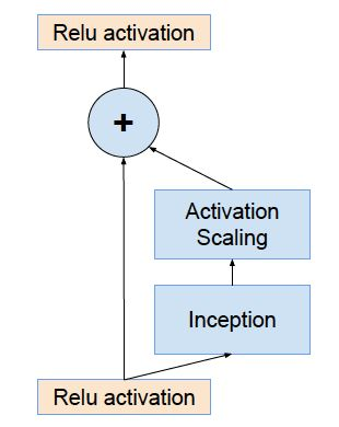
The code demonstrates this more clearly:

def forward(self, x):    out = self.conv2d(x)  # This can be a convolution layer, an Inception module, or any sub-network    out = out * self.scale + x  # Multiply by a scaling factor before adding    out = self.relu(out)    return out

Introducing scale can solve this issue, and doing so does not reduce accuracy while making the network more stable.

5. GoogLeNet Tensorflow2.0 Practical Application

GitHub link: https://github.com/freeshow/ComputerVisionStudy

6. Reference Links

• https://my.oschina.net/u/876354/blog/1637819
• https://blog.csdn.net/abc13526222160/article/details/95472241
• https://juejin.im/post/5db90c41e51d4529e9478258