Simple Preferences of Neural Networks

I started to get in touch with deep learning in November 2017, and it has been exactly five years. I joined Shanghai Jiao Tong University in October 2019, and it has been three years, just at the first stage of assessment. On August 19, 2022, I gave a keynote speech at the first China Machine Learning and Scientific Applications Conference, summarizing my research over the past five years and looking forward to future directions. This article is a summary of the theoretical research from that report (with some expansion). The video link of the report can be found at: https://www.bilibili.com/video/BV1eB4y1z7tL/

I originally researched computational neuroscience, which, broadly speaking, is to understand how the brain works from a mathematical perspective. Specifically, my research dealt with processing spike data generated by high-dimensional neural networks, trying to understand how these signals process input signals. However, the brain is too complex, and the dimensions are too high; our ordinary brain has about 100 billion neurons, and each neuron has signal transmission with thousands of other neurons. I had little confidence in processing such data, and at that stage, I happened to read an article that suggested using current computational neuroscience research methods to study computer chips, concluding that these methods could not help us understand the working principles of chips. Another aspect that troubled me was that we not only know little about the brain but also find it very difficult to obtain data from the brain. Therefore, we thought at the time, is it possible to find a simple network model that can achieve complex functions while having little understanding of it, and use our research on it to inspire our study of the brain?

At the end of 2017, deep learning had become very popular, especially since my classmates had already been exposed to deep learning for some time, so we quickly learned about deep learning. Its structure and training seemed simple enough, yet it was powerful, and the relevant theories were still in their infancy. Therefore, my first thought of entering deep learning was to treat it as a simple model for studying the brain. Clearly, under this positioning of “brain-like research“, we are concerned with the basic research of deep learning. Here, I want to distinguish between the “theory” of deep learning and “basic research.” I believe that “theory” gives people a feeling of being all about formulas and proofs. In contrast, “basic research” sounds broader; it can include “theory” as well as important phenomena, intuitive explanations, laws, empirical principles, etc. This distinction is merely a subjective one; in practice, we do not really make such a detailed distinction when discussing them. Although we use deep learning as a model to study why the brain has such complex learning abilities, there are still significant differences between the brain and deep learning. Moreover, from the perspectives of knowledge reserve, ability, and time, it is challenging for me to delve into these two fields that currently seem quite distant simultaneously.

So, I chose to fully shift to deep learning, focusing on the question of what characteristics deep learning as an algorithm has. The “no free lunch” theorem tells us that when considering the average performance across all possible datasets, all algorithms are equivalent, meaning that no single algorithm is universal. We need to clarify what data deep learning algorithms are suitable for and what data they are not suitable for. In fact, the theory of deep learning is not in its infancy; since the mid-20th century, when it began to develop, relevant theories have already started, and there have been some important results. However, overall, it is still in its early stages. For me, this is an extremely challenging question. Thus, I turned to viewing deep learning as a kind of “toy“, adjusting various hyperparameters and different tasks to observe what “natural phenomena” it would produce. The goals set were no longer grand but simply interesting; discovering interesting phenomena and explaining them, perhaps even using them to guide practical applications. Under these understandings, we began with some interesting phenomena in deep neural network training. Personally, I started learning Python and TensorFlow from scratch, specifically by finding several codes online and copying them while trying to understand.

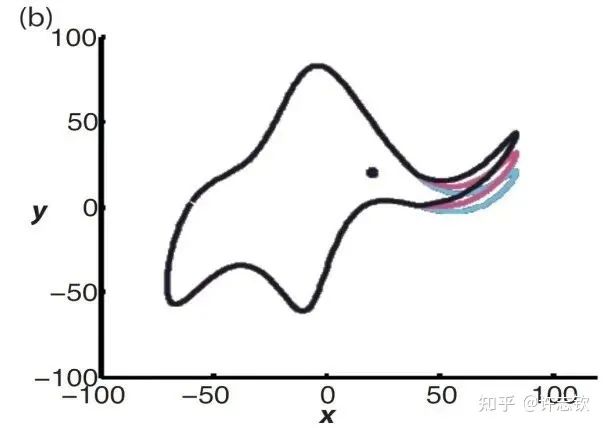
In traditional learning theory, the number of model parameters is an important indicator of model complexity. As the complexity of the model increases, its ability to fit the training data enhances, but it also leads to overfitting issues on the test set. Von Neumann once famously said, give me four parameters, and I can fit an elephant; five parameters can make the elephant’s trunk move.

Therefore, researchers related to traditional modeling often calculate the number of parameters when using neural networks and intentionally use networks with fewer parameters to avoid overfitting. However, today, the great success of neural networks is largely due to the use of ultra-large-scale networks. The number of parameters in the network often far exceeds the number of samples, yet it does not overfit as traditional learning theory predicts. This is the generalization puzzle that has received great attention in recent years. In fact, in 1995, Leo Breiman pointed out this problem in an article. Today, as neural networks become increasingly popular and important, this puzzle becomes even more significant. We can ask: Are neural networks with a large number of parameters really complex?

The answer is yes! The theoretical work from the late 1980s proved that when two-layer neural networks (with non-polynomial activation functions) are wide enough, they can approximate any continuous function with arbitrary precision, which is the famous “universal approximation” theorem. In reality, we should ask a more meaningful question: Is the neural network really complex during actual training? The solutions proven by approximation theory are almost impossible to encounter during actual training. Actual training requires setting initial values, optimization algorithms, network structures, and other hyperparameters. For our practical guidance, we cannot consider generalization issues without these factors, as generalization itself relies on actual data.

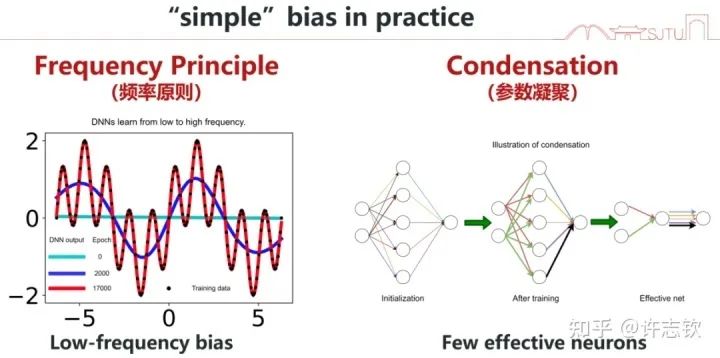
In the process of learning and training neural networks, we can easily find that the training of neural networks follows certain rules. In our research, there are two interesting phenomena, and in studying and explaining them, we found them to be quite meaningful. I will briefly introduce them first and then detail them separately. First, we found that neural networks often learn low frequencies first while fitting data and then gradually learn high frequencies. We named this phenomenon the Frequency Principle (F-Principle) [1, 2], and other works refer to it as Spectral bias. Second, we found that during the training process, many neurons’ input weights (vectors) tend to maintain consistent directions. We call this the Cohesion Phenomenon. Neurons with identical input weights process inputs in the same way, allowing them to be simplified into a single neuron, meaning a large network can be simplified into a smaller network [3, 4]. Both phenomena reflect an implicit simple preference in neural networks during training, either a low-frequency preference or an effective small network preference. The low-frequency preference is very common, while the small network preference only appears as a feature in non-linear training processes.

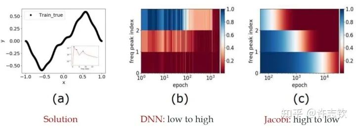
When I initially reported work related to the Frequency Principle, teachers and students in computational mathematics were very interested because, in traditional iterative formats, such as Jacobi iteration, low frequencies converge very slowly. The multigrid method effectively solves this problem. In our experiments, we also verified that neural networks and Jacobi iterations have completely different frequency convergence orders when solving PDEs (as shown below) [2, 5].

How widespread is the Frequency Principle? The Frequency Principle was first discovered in the fitting of one-dimensional functions. During parameter tuning, I found that neural networks seem to always capture the contour information of the target function first and then the details. Frequency is a quantity very suitable for characterizing contours and details. Thus, we observed the learning process of neural networks in frequency space and found a very clear order from low frequency to high frequency.

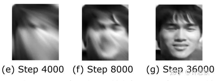
For two-dimensional functions, using images as an example, neural networks learn the mapping from two-dimensional positions to grayscale values. During the training process, the neural networks gradually remember more details.

For higher-dimensional examples, Fourier transforms are difficult, which is also a reason why it is not easy to discover the frequency principle in high-dimensional image classification tasks. Our contribution also includes demonstrating through an example that research on simple low-dimensional problems can inspire foundational research in deep learning. More needs to be said about the frequency in high dimensions. Essentially, high frequency refers to output being very sensitive to input changes. For example, in image classification tasks, when an image is modified slightly, the output changes significantly. This is exactly what is meant by adversarial examples. Regarding validating the frequency principle in high dimensions, we used dimensionality reduction and filtering methods. A series of experiments have verified that the frequency principle is a widely existing phenomenon.

Why does the Frequency Principle exist? In fact, most signals in nature have a characteristic where intensity decreases with increasing frequency. Generally, the functions we encounter also exhibit decay characteristics in frequency space, especially the smoother the function, the faster the decay. Even the common ReLU function in frequency space decays quadratically with respect to frequency. In gradient descent calculations, it is easy to see that low-frequency signals contribute more to the gradient than high frequencies, so gradient descent naturally aims to eliminate low-frequency errors as the primary goal [2]. For general networks, we have qualitative theoretical proofs [6], and for networks in the linear NTK region, we have a strict linear frequency principle model that reveals the mechanism of frequency decay [7, 8, 9]. With this understanding, we can also construct some examples to accelerate the convergence of high frequencies, such as adding the output derivative with respect to input in the loss function, since differentiation in frequency space is equivalent to multiplying the corresponding frequency by its intensity, which can alleviate high-frequency difficulties. This is common in solving PDEs.

Does understanding the Frequency Principle help us understand neural networks? We provide two examples. The first is understanding the early stopping technique. In actual training, it is generally found that the point of best generalization is not the lowest training error; it usually requires stopping training early when the training error has not dropped too low. Actual data are mostly dominated by low frequencies and generally contain noise. Noise has relatively little impact on low frequencies but has a greater impact on high frequencies, and neural networks learn low frequencies first in the learning process. Therefore, early stopping can avoid learning too much contaminated high frequency, resulting in better generalization performance. Another example is that we find that the mapping from images to categories in image classification problems is usually also dominated by low frequencies, which can explain its good generalization. However, for odd functions defined in d-dimensional space, each dimension’s value can only be 1 or -1. Clearly, any disturbance in one dimension will cause a significant change in the output. This function can be proven to be high frequency dominant, and in actual training, neural networks have no predictive capability in this problem. We also used the frequency principle to explain why deep networks can accelerate training in experiments; the core reason is that deeper networks turn the target function into a lower frequency function, making learning easier [10].

Besides understanding, can the Frequency Principle provide guidance for the design and use of neural networks? The Frequency Principle reveals the existence of high-frequency disasters in neural networks, which has also attracted the attention of many researchers, including solving PDEs, generating images, fitting functions, etc. The training and generalization difficulties caused by high-frequency disasters are hard to alleviate through simple parameter tuning. Our group proposed a multi-scale neural network method to accelerate high-frequency convergence [11]. The basic idea is to stretch the target function radially at different scales, attempting to stretch different frequency components into consistent low frequencies for uniform rapid convergence. Implementation is also very easy, requiring only multiplying the inputs of the neurons in the first hidden layer by some fixed coefficients. Some of our work has found that adjusting activation functions significantly impacts network performance [12], and using sine and cosine functions as the basis for the first hidden layer can yield good results [13]. This algorithm has been adopted by Huawei’s MindSpore. The idea of radial stretching has also been adopted in many other algorithms, including the well-known NerF (Neural Radiance Fields) in image rendering.

The Frequency Principle still has many unresolved questions that need to be explored. In non-gradient descent training processes, such as how to prove frequency decay in particle swarm optimization [14]? How to theoretically demonstrate the acceleration effect of multi-scale neural networks on high frequencies? Are there more stable and faster high-frequency acceleration algorithms? Can wavelets describe different local frequency characteristics more finely, and can we use wavelets to understand the training behavior of neural networks in more detail? How do data volume, network depth, and loss functions affect the frequency principle? The frequency principle can guide the theoretical design of algorithms and provide a “macroscopic” description of training laws. For the “microscopic” mechanisms, we need further research. Even for the learning process from low frequency to high frequency, the evolution of parameters can be very different. For example, a function can be represented by one neuron or by ten neurons (with each neuron’s output weight being 1/10 of the original output weight). From the perspective of frequency regarding the input-output function, there is no difference between these two representations. Which representation will the neural network choose, and what differences do these representations have? Next, we will look more closely at the phenomena in parameter evolution.

To introduce the parameter cohesion phenomenon, we need to discuss the expression of a two-layer neural network.

W is the input weight, which extracts the components of the input in the direction of the weight through the inner product, which can be understood as a feature extraction method. Adding a bias term, and then passing through a nonlinear function (also called an activation function), completes the calculation of a single neuron, and then all neurons’ outputs are weighted and summed. For convenience, we denote

For the ReLU activation function, we can understand each neuron’s features by considering the angles of input weights and the amplitude of neurons: , where . Considering the two-layer neural network above to fit four one-dimensional data points, combining input weights and bias terms, the direction we are concerned about is two-dimensional, so we can represent its direction using angles. The diagram below shows the fitting results of the neural network under different initializations (first row) and the feature distribution before training (cyan) and after training (red) (second row).

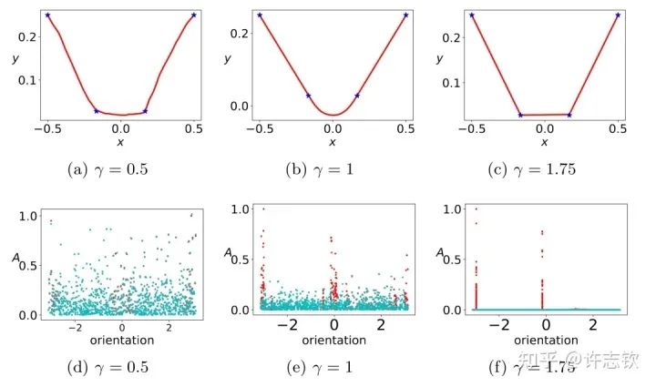
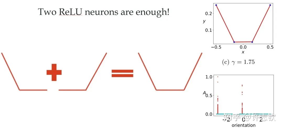
Clearly, as the initialization scale decreases (from left to right, the initialization scale continues to decrease), the fitting results of the neural network vary greatly. In terms of feature distribution, when the scale is large (using NTK initialization here), the neural network features remain almost unchanged, similar to linear models like random features. However, as the initialization decreases, a significant change in features appears during the training process. The most interesting thing is that these feature directions cluster into two primary directions. We call this phenomenon parameter cohesion. Numerous practical problems tell us that neural networks outperform linear methods significantly. What benefits does the non-linear process of parameter cohesion present? The extreme example of cohesion shown below illustrates that for a randomly initialized network, after a brief training, the input weights of each hidden layer neuron are completely consistent, allowing this network to be equivalent to a small network with only one hidden layer neuron. Generally, neurons will cluster into multiple directions.

Reflecting on the generalization puzzle we mentioned earlier and the initial question we posed, “Is the neural network really complex during actual training?” In the case of parameter cohesion, for a network that appears to have many parameters on the surface, we naturally want to ask: How many effective parameters does the neural network actually have? For example, in the case of the two-layer neural network clustering in two directions we saw earlier, the effective neurons of this network are only two. Therefore, cohesion can effectively control the model’s complexity based on the actual data fitting needs.

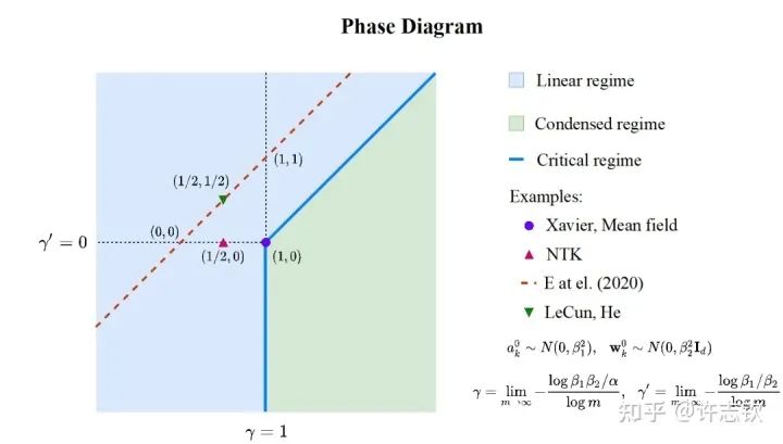
Previously, we presented the cohesion phenomenon through a simple example. The next important question is: Is parameter cohesion a common phenomenon in non-linear processes? Inspired by phase diagrams in statistical mechanics, we experimentally discovered and theoretically derived the phase diagram for two-layer infinite-width ReLU neural networks. Based on different initialization scales, using the relative distance of parameters before and after training as a criterion in the infinite-width limit, the phase diagram divides the dynamics into linear, critical, and cohesive three states (dynamical regime). A series of theoretical studies in the field (including NTK, mean-field, etc.) can be found in corresponding positions in our phase diagram [3].

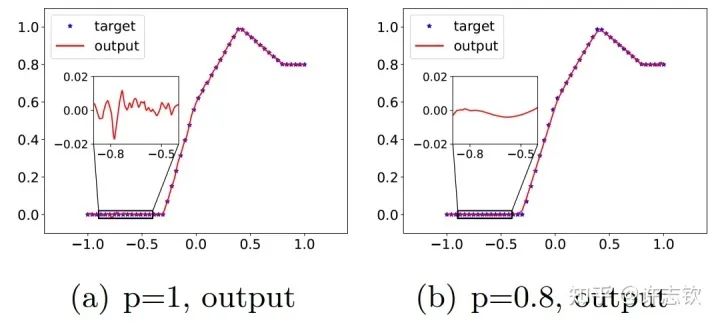
In a three-layer infinite-width fully connected network [15], we experimentally proved that parameter cohesion is a common phenomenon in all non-linear regions. Theoretically, we demonstrated that when the initialization scale is sufficiently small, cohesion will occur in the initial training phase [4]. Interestingly, when studying the implicit regularization of the Dropout algorithm, we found that the Dropout algorithm significantly promotes the formation of parameter cohesion. The idea of the Dropout algorithm, proposed by Hinton, is a common technique in training neural networks, where neurons are retained with a certain probability p, which significantly helps improve generalization. First, let’s look at the fitting results. The left image below is an example without Dropout, where we can see significant small-scale fluctuations in the fitted function. The right image shows the results with Dropout, where the fitted function is much smoother.

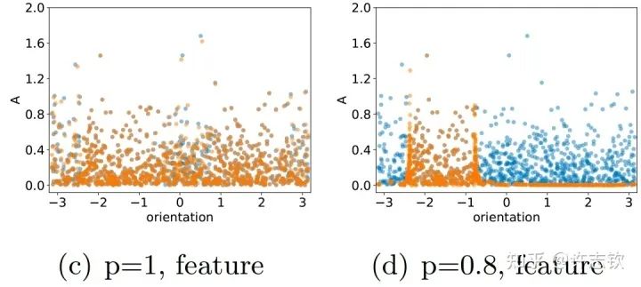
Looking closely at their feature distributions, we can see that the distributions before training (blue) and after training (orange) with Dropout are significantly different, showing a clear cohesion effect, where the effective parameters become fewer, and the function complexity correspondingly becomes simpler and smoother.

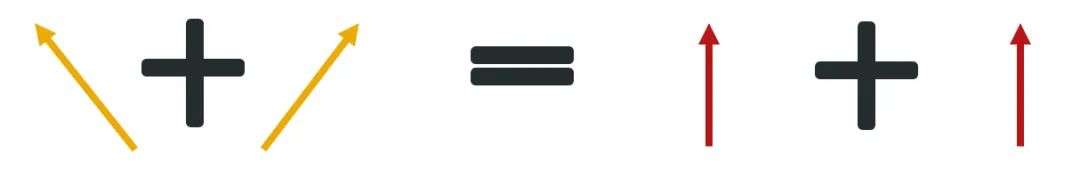
Furthermore, we analyze why Dropout brings about the cohesion effect. We find that Dropout training results in a special implicit regularization effect. We use the following example to understand this effect. Both the yellow and red cases can combine into the same vector, but Dropout requires the sum of the squared norms of the two sub-vectors to be minimized. Clearly, this can only happen when the two vectors’ directions are consistent and completely equal; for w, this is cohesion.

At this point, we have discussed how parameter cohesion reduces the effective scale of neural networks. So why don’t we directly train a small-scale network? What are the differences between large and small networks? First, we use two-layer networks of different widths to fit the same batch of data. The diagram below shows their loss descent process.

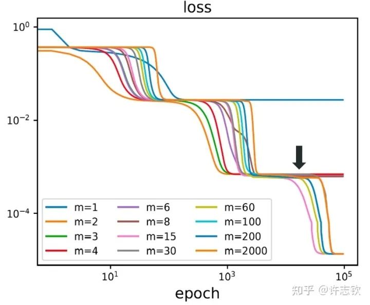
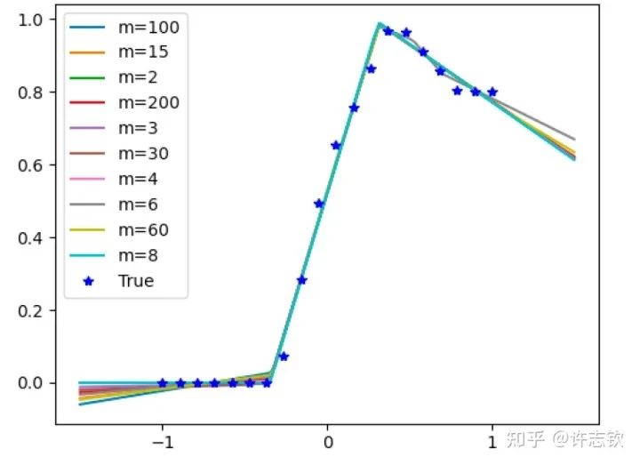
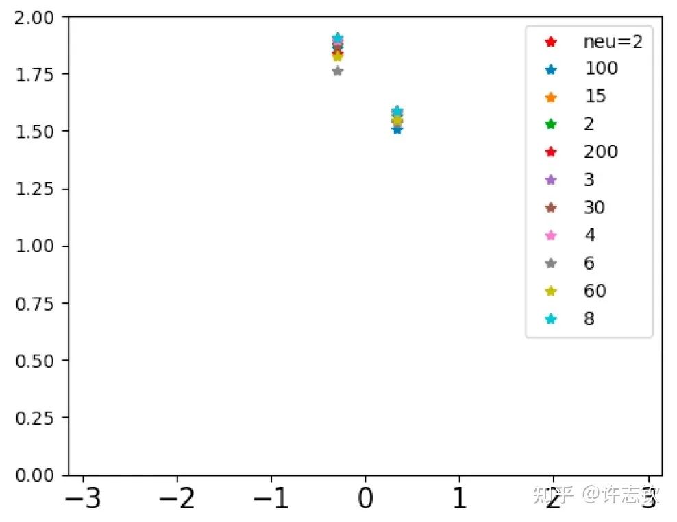
The loss functions of networks of different widths exhibit a high degree of similarity, and they tend to pause at common points. What similarities exist at these common steps? The left image below shows that for the steps indicated by arrows, the output functions of networks of different widths are very close. Furthermore, looking at their feature maps (bottom right), they exhibit strong cohesion phenomena. These reflect their similarities.

If we observe their loss graphs closely, we can find that as the width increases, the loss function of the network is more likely to decrease. For example, at the point indicated by the arrow, the relatively small network remains at a plateau, while the larger network’s loss continues to decrease. Experimentally, we can see that while large networks condense into effective small networks, they seem to be easier to train than small networks. How can we explain the similarities of networks of different widths and the advantages of large networks? In a gradient descent training process, the occurrence of plateaus is likely due to the training path experiencing a saddle point (a local extremum where there are both ascending and descending directions). Different widths of networks seem to experience the same saddle point. However, networks with different parameter counts have their saddle points located in different dimensional spaces; how can they be at the same point?

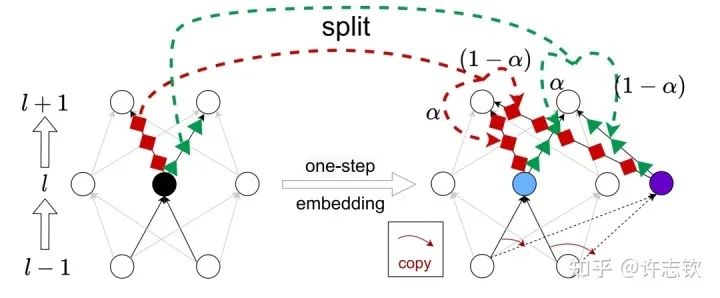
We proved that the extreme points of the loss landscape of networks of different widths exist under an embedding principle (Embedding Principle) [16], meaning that the loss landscape of one neural network “contains” all critical points (including saddle points, local optima, and global optima) of loss landscapes of all narrower neural networks. Simply put, when a network processes critical points, through a specific embedding method, it can be embedded into a wider network, maintaining the network output unchanged and keeping the wider network at critical points. The simplest embedding method is the inverse process of cohesion; for example, the diagram below shows an embedding method in one step. More general embedding methods are discussed in detail in our article in the first issue of the Journal of Machine Learning [17].

The embedding principle reveals the similarities of networks of different widths and also provides a means to study their differences. Since there are free parameters during the embedding process, the greater the degree of degeneration at the critical points of the larger network. Likewise, if a critical point from a larger network originates from the embedding of a simpler network’s critical point, its degree of degeneration is also greater (intuitively understood as occupying more space). We can speculate that these simpler critical points are more likely to be learned.

Additionally, we theoretically proved that during the embedding process, the descending and ascending directions near critical points do not decrease. This tells us that if a saddle point is embedded into a larger network, it cannot become a minimum point. However, if a minimum point is embedded into a larger network, it is likely to become a saddle point, producing more descending directions. We also experimentally demonstrated that the embedding process generates more descending directions.

Therefore, we have reason to believe that even though large networks condense into effective small networks, they are easier to train than small networks. In other words, large networks can control model complexity (which may lead to better generalization) while also making training easier. Our work also discovered the embedding principle of the loss landscape in the depth of neural networks [18]. Regarding the cohesion phenomenon, many questions remain to be explored. Here are some examples. Besides initial training, what mechanisms generate cohesion during the training process? Do different network structures exhibit cohesion phenomena? What is the relationship between the process of cohesion and the frequency principle? How can cohesion be quantitatively linked to generalization?

Over the past five years, in foundational research on deep learning, we have primarily focused on two phenomena: the Frequency Principle and parameter cohesion. From discovering them, realizing their interest, to explaining them, and to some extent, understanding other aspects of deep learning and designing better algorithms based on this work. In the next five years, we will delve deeper into foundational research in deep learning and AI for Science.

References

[1] Zhi-Qin John Xu*, Yaoyu Zhang, and Yanyang Xiao, Training behavior of deep neural network in frequency domain, arXiv preprint: 1807.01251, (2018), ICONIP 2019.

[2] Zhi-Qin John Xu*, Yaoyu Zhang, Tao Luo, Yanyang Xiao, Zheng Ma, Frequency Principle: Fourier Analysis Sheds Light on Deep Neural Networks, arXiv preprint: 1901.06523, Communications in Computational Physics (CiCP).

[3] Tao Luo#, Zhi-Qin John Xu #, Zheng Ma, Yaoyu Zhang*, Phase diagram for two-layer ReLU neural networks at infinite-width limit, arxiv 2007.07497 (2020), Journal of Machine Learning Research (2021)

[4] Hanxu Zhou, Qixuan Zhou, Tao Luo, Yaoyu Zhang*, Zhi-Qin John Xu*, Towards Understanding the Condensation of Neural Networks at Initial Training. arxiv 2105.11686 (2021), NeurIPS2022.

[5] Jihong Wang, Zhi-Qin John Xu*, Jiwei Zhang*, Yaoyu Zhang, Implicit bias in understanding deep learning for solving PDEs beyond Ritz-Galerkin method, CSIAM Trans. Appl. Math.

[6] Tao Luo, Zheng Ma, Zhi-Qin John Xu, Yaoyu Zhang, Theory of the frequency principle for general deep neural networks, CSIAM Trans. Appl. Math., arXiv preprint, 1906.09235 (2019).

[7] Yaoyu Zhang, Tao Luo, Zheng Ma, Zhi-Qin John Xu*, Linear Frequency Principle Model to Understand the Absence of Overfitting in Neural Networks. Chinese Physics Letters, 2021.

[8] Tao Luo*, Zheng Ma, Zhiwei Wang, Zhi-Qin John Xu, Yaoyu Zhang, An Upper Limit of Decaying Rate with Respect to Frequency in Deep Neural Network, To appear in Mathematical and Scientific Machine Learning 2022 (MSML22),

[9] Zhi-Qin John Xu*, Hanxu Zhou, Deep frequency principle towards understanding why deeper learning is faster, AAAI 2021, arxiv 2007.14313 (2020)

[10] Ziqi Liu, Wei Cai, Zhi-Qin John Xu*, Multi-scale Deep Neural Network (MscaleDNN) for Solving Poisson-Boltzmann Equation in Complex Domains, arxiv 2007.11207 (2020) Communications in Computational Physics (CiCP).

[11] Xi-An Li, Zhi-Qin John Xu*, Lei Zhang, A multi-scale DNN algorithm for nonlinear elliptic equations with multiple scales, arxiv 2009.14597, (2020) Communications in Computational Physics (CiCP).

[12] Xi-An Li, Zhi-Qin John Xu, Lei Zhang*, Subspace Decomposition based DNN algorithm for elliptic type multi-scale PDEs. arxiv 2112.06660 (2021)

[13] Yuheng Ma, Zhi-Qin John Xu*, Jiwei Zhang*, Frequency Principle in Deep Learning Beyond Gradient-descent-based Training, arxiv 2101.00747 (2021).

[14] Hanxu Zhou, Qixuan Zhou, Zhenyuan Jin, Tao Luo, Yaoyu Zhang, Zhi-Qin John Xu*, Empirical Phase Diagram for Three-layer Neural Networks with Infinite Width. arxiv 2205.12101 (2022), NeurIPS2022.

[15] Yaoyu Zhang*, Zhongwang Zhang, Tao Luo, Zhi-Qin John Xu*, Embedding Principle of Loss Landscape of Deep Neural Networks. NeurIPS 2021 spotlight, arxiv 2105.14573 (2021)

[16] Zhongwang Zhang, Zhi-Qin John Xu*, Implicit regularization of dropout. arxiv 2207.05952 (2022)

[17] Zhiwei Bai, Tao Luo, Zhi-Qin John Xu*, Yaoyu Zhang*, Embedding Principle in Depth for the Loss Landscape Analysis of Deep Neural Networks. arxiv 2205.13283 (2022)

About Us