Click on the above “Beginner Learning Vision” to choose to add Starred or “Top”

Heavy content delivered at the first time

Author丨Li Ming Huai Jin

Source｜https://zhuanlan.zhihu.com/p/80361782

Editor丨Extreme City Platform

Extreme City Guide

This article first defines the concept of Convolutional Neural Networks, briefly introduces several common optimization methods, and discusses the author’s experiences in this field.

Introduction

Upon seeing this title, many friends must be unable to help but say, “No way, is it another clichéd topic that has been written tens of thousands of times?” accompanied by a dog head emoji. I am also quite helpless, wanting to write but having no solid content, I can only pick and choose. However, this article still has different content from other similar topics, and I believe it can bring some gains to everyone~

Convolution is one of the core computations of neural networks, and its breakthrough in computer vision has led the wave of deep learning. The variations of convolution are rich, and the computational complexity is high; most of the time during neural network operation is spent on convolution calculations. As the development of network models continues to increase network depth, optimizing convolution calculations becomes particularly important.

With the development of technology, researchers have proposed various optimization algorithms, including Im2col, Winograd, etc. This article first defines the concept of Convolutional Neural Networks, briefly introduces several common optimization methods, and discusses the author’s experiences in this field.

• Most of the time is spent on convolution calculations Link: https://arxiv.org/abs/1807.11164 ,

• Im2col Link: https://www.mathworks.com/help/images/ref/im2col.html ,

• Winograd Link: https://www.intel.ai/winograd/#gs.avmb0n

Concept of Convolutional Neural Networks

The concept of Convolutional Neural Networks (CNN) extends from the convolution in the field of signal processing. The convolution in signal processing is defined as

(1)

Due to symmetry Convolution calculations are intuitively difficult to understand, and their visualization is shown in Figure 1. The red slider in the figure moves and is multiplied with the blue square to form a triangular pattern, which is the convolution result (𝑓∗𝑔)(𝑡) at various points.

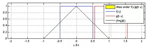
Figure 1: Convolution in Signal Processing

• Convolution in Signal Processing Link: https://jackwish.net/convolution-neural-networks-optimization.html

The discrete form of formula 1 is

(2)

Extending this convolution into two-dimensional space gives the convolution in neural networks, which can be abbreviated as

(3)

Where 𝑆 is the convolution output, 𝐼 is the convolution input, and 𝐾 is the convolution kernel. The dynamic visualization of this calculation can refer to conv_arithmetic, which will not be introduced here.

• conv_arithmetic Link: https://github.com/vdumoulin/conv_arithmetic

When applied to computer vision for processing images, the channels of the image can simply stack the two-dimensional convolutions, i.e.

(4)

Where 𝑐c is the input channel. This is the computation of applying two-dimensional convolutions in three-dimensional tensors.

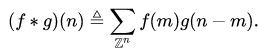
Many times, the formula description seems not very intuitive; Figure 2 is a visualization of stacked two-dimensional convolutions. Among them, the labels related to input, output, and convolution kernels are prefixed with I, O, K. In addition, the color coding for the output, input, and convolution kernel in this article is generally: orange, yellow, and green.

Figure 2: Definition of Convolution Calculation

When the memory layout of the tensor is NHWC, the corresponding pseudocode for convolution calculations is as follows. The outer three loops traverse each data point of the output 𝐶C; for each output data, the inner three loops need to accumulate the sum to obtain (dot product).

for (int oh = 0; oh < OH; oh++) {
for (int ow = 0; ow < OW; ow++) {
    for (int oc = 0; oc < OC; oc++) {
      C[oh][ow][oc] = 0;
      for (int kh = 0; kh < KH, kh++){
        for (int kw = 0; kw < KW, kw++){
          for (int ic = 0; ic < IC, ic++){
            C[oh][ow][oc] += A[oh+kh][ow+kw][ic] * B[kh][kw][ic];
          }
        }
      }
    }
  }
}

Similar to the optimization methods for matrix multiplication, we can also apply basic optimization operations such as vectorization, parallelization, and loop unrolling to this computation. The problem with convolution is that its 𝐾𝐻 and 𝐾𝑊 generally do not exceed 5, making it difficult to vectorize, while the computation of features has data reuse in spatial dimensions. The complexity of this computation has led to several optimization methods; below we introduce several.

• Optimization methods for matrix multiplication Link: https://jackwish.net/gemm-optimization.html

Im2col Optimization Algorithm

As an early deep learning framework, Caffe implemented convolution based on the Im2col method, which is still one of the important optimization methods for convolution today.

Im2col is the process of converting an image into a matrix column in the field of computer vision. From the introduction in the previous section, it can be seen that the computation of two-dimensional convolution is relatively complex and difficult to optimize. Therefore, in the early development of deep learning frameworks, Caffe used the Im2col method to convert three-dimensional tensors into two-dimensional matrices, thereby fully utilizing the already optimized GEMM libraries to accelerate convolution calculations for various platforms. Finally, the two-dimensional matrix results obtained from matrix multiplication are converted back to three-dimensional matrices using Col2im.

• Caffe Link: http://caffe.berkeleyvision.org/

• Caffe uses the Im2col method to convert three-dimensional tensors into two-dimensional matrices Link: https://github.com/Yangqing/caffe/wiki/Convolution-in-Caffe:-a-memo

Algorithm Process

Unless otherwise specified, the memory layout form adopted in this article is NHWC. Other memory layouts and specific converted matrix shapes may vary slightly, but do not affect the description of the algorithm itself.

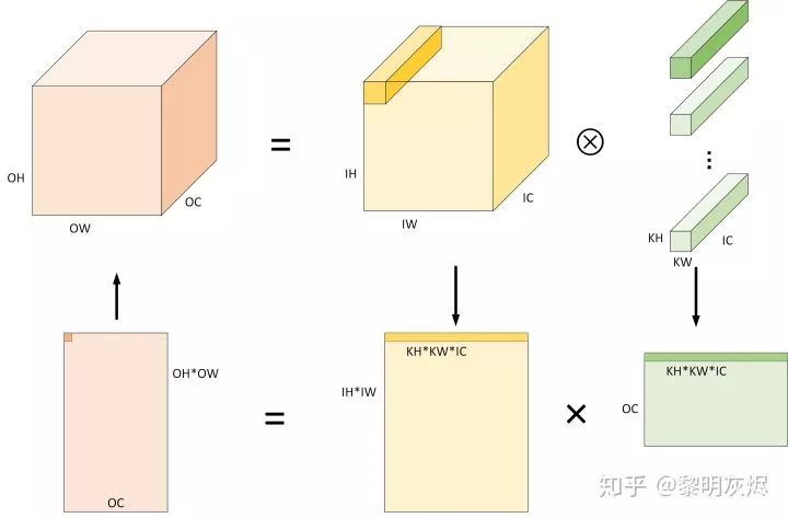
Figure 3: The Process of Computing Convolution Using Im2col Algorithm

Figure 3 is an example of the process of calculating convolution using the Im2col algorithm. The specific process includes (for simplicity, ignoring the case of Padding, i.e., assuming 𝑂𝐻=𝐼𝐻,𝑂𝑊=𝐼𝑊):

1. Expand the input from 𝐼𝐻×𝐼𝑊×𝐼𝐶 into a two-dimensional matrix of shape (𝑂𝐻×𝑂𝑊)×(𝐾𝐻×𝐾𝑊×𝐼𝐶) based on the convolution calculation characteristics. Clearly, the memory space used after conversion is approximately 𝐾𝐻∗𝐾𝑊−1 times more than the original input.

2. The shape of the weights is generally a four-dimensional tensor of 𝑂𝐶×𝐾𝐻×𝐾𝑊×𝐼𝐶, which can be treated directly as a two-dimensional matrix of shape (𝑂𝐶)×(𝐾𝐻×𝐾𝑊×𝐼𝐶).

3. For the two prepared two-dimensional matrices, run matrix multiplication using (𝐾𝐻×𝐾𝑊×𝐼𝐶) as the dimension for accumulation, which can yield the output matrix (𝑂𝐻×𝑂𝑊)×(𝑂𝐶). This process can be accomplished using various optimized BLAS (Basic Linear Algebra Subprograms) libraries.

4. The output matrix (𝑂𝐻×𝑂𝑊)×(𝑂𝐶) in terms of memory layout is the expected output tensor 𝑂𝐻×𝑂𝑊×𝑂𝐶.

The cost of using GEMM for convolution calculations with Im2col is the additional memory overhead. This is because in the original convolution calculation, the convolution kernel slides over the input to compute the output, and adjacent output calculations spatially reuse certain inputs and outputs. However, when using Im2col to unfold three-dimensional tensors into two-dimensional matrices, the data that could originally be reused is flattened into the matrix, leading to 𝐾𝐻∗𝐾𝑊−1 copies of the input data.

When the convolution kernel size 𝐾𝐻×𝐾𝑊 is 1×1, the 𝐾𝐻 and 𝐾𝑊 in the above steps can be eliminated, i.e., the input shape after transformation is (𝑂𝐻×𝑂𝑊)×(𝐼𝐶), the convolution kernel shape is (𝑂𝐶)×(𝐼𝐶), and the convolution calculation degenerates into matrix multiplication. It is noteworthy that for this case, the Im2col process does not actually change the shape of the input, so the matrix multiplication operation can run directly on the original input, thus saving the memory organization process (i.e., steps 1, 2, and 4 in the above).

Memory Layout and Convolution Performance

The memory layout of convolutions in neural networks mainly includes NCHW and NHWC. Different memory layouts affect the patterns of memory access during computation, especially during matrix multiplication. This section analyzes the relationship between computational performance and memory layout when using the Im2col optimization algorithm.

• Especially during matrix multiplication Link: https://jackwish.net/gemm-optimization.html

After completing the Im2col transformation, the input matrix and convolution kernel matrix for running matrix multiplication are obtained. Applying common data partitioning, vectorization, and other optimization methods used in matrix calculations (for related definitions, please refer toGeneral Matrix Multiplication (GEMM) Optimization Algorithm), this section focuses on analyzing the impact of different memory layouts on performance in this scenario.

• General Matrix Multiplication (GEMM) Optimization Algorithm Link: https://jackwish.net/gemm-optimization.html

First, consider the NCHW memory layout, mapping the convolution of the NCHW memory layout to matrix multiplication 𝐶=𝐴𝐵, where 𝐴 is the convolution kernel (filter), and 𝐵 is the input (input), with the dimensions of each matrix shown in Figure 4. The 𝑀,𝑁,𝐾 in the figure are used to label matrix multiplication, i.e.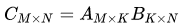, while also marking their relationships with various dimensions in convolution calculations.

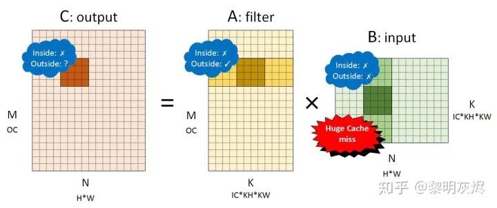
Figure 4: Matrix Multiplication Corresponding to Convolution in NCHW Memory Layout

After partitioning this matrix, we analyze the performance of locality in detail, marked in Figure 4. Among them, Inside indicates the locality within the 4×4 small block matrix multiplication, while Outside indicates the locality between small blocks in the dimension reduction direction.

• For the output, the locality within the small block is poor because each vectorized load will load four elements, and each load will incur a cache miss. The external performance depends on the global computation direction—row-major has better locality, while column-major has poorer locality. The behavior of the output is not the end of the discussion here, as it does not have memory reuse.

• For the convolution kernel, the locality within the small block is poor, similar to the output. When a cache miss occurs during small block loading, the processor will load a cache line at once, allowing subsequent small block accesses to hit the cache until the entire cache line is hit before entering the next cache line range. Therefore, the external locality of small blocks is good.

• For the input, the locality within the small block also performs poorly. However, unlike the convolution kernel, the data loaded into the cache from the cache line in the small block due to cache misses will only be used once because, in this memory layout, the next small block’s address range generally exceeds a cache line. Therefore, nearly every memory load for the input will incur a cache miss—the cache does not accelerate, and every access needs to fetch data from memory.

Therefore, when processing convolution calculations with Im2col, the NCHW layout is not memory-friendly.

Figure 5 is an example of the NHWC memory layout. It is noteworthy that the tensors represented by matrices 𝐴 and 𝐵 in NHWC and NCHW have been swapped—𝑂𝑢𝑡𝑝𝑢𝑡=𝐼𝑛𝑝𝑢𝑡×𝐹𝑖𝑙𝑡𝑒𝑟 (the swap is merely to avoid drawing another figure). The specific splitting method remains the same and is precisely the steps described in the previous section to construct the matrices.

Figure 5: Matrix Multiplication Corresponding to Convolution in NHWC Memory Layout

Similarly, analyzing the memory performance of the three tensors shows:

• For the output, NHWC performs similarly to NCHW.

• For the input, the internal locality of small blocks performs poorly because several vector loads will incur cache misses; however, the external locality performs well because the memory used in the sliding dimension is contiguous. This performance is similar to that of the convolution kernel in NCHW, and overall, it is a memory layout that is more cache-friendly.

• For the convolution kernel, NHWC’s situation is similar to that of the input in NCHW, where both internal and external locality of small blocks are poor.

The cache performance of the convolution kernel in both memory layouts is not an issue because the convolution kernel remains unchanged during operation. The memory layout of the convolution kernel can be rearranged during the model loading phase, making it friendly to caches in the memory outside small blocks (for example, converting the layout from (𝐼𝐶×𝐾𝐻×𝐾𝑊)×(𝑂𝐶) to (𝑂𝐶)×(𝐼𝐶×𝐾𝐻×𝐾𝑊)). It is worth noting that the operation of general frameworks or engines can be divided into at least two phases: preparation and execution. Some preprocessing tasks of models can be completed in the preparation phase, such as rearranging the memory layout of the convolution kernel, which remains unchanged during the execution phase.

Therefore, when using the Im2col method for calculations, the overall memory performance depends on the input situation, i.e., the NHWC memory layout is more friendly than the NCHW memory layout. An experiment during our practical process indicated that for a convolution with a 1×1 convolution kernel, when similar optimization methods are applied, switching from NCHW to NHWC can reduce the cache miss rate from about 50% to around 2%. Such an improvement can significantly enhance the performance of software (specifically referring to cases without specially designed matrix multiplication optimization methods).

Spatial Packing Optimization Algorithm

Im2col is a relatively straightforward convolution optimization algorithm, and without careful handling, it can lead to significant memory overhead. Spatial packing is an optimization algorithm similar to memory reorganization in matrix multiplication.

• Memory Reorganization in Matrix Multiplication Link: https://github.com/flame/how-to-optimize-gemm/wiki#packing-into-contiguous-memory

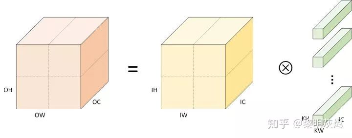
Figure 6: Division of Computation by Spatial Packing Optimization Algorithm

The spatial packing optimization algorithm is a divide-and-conquer method—it divides the convolution computation into several parts based on spatial characteristics and processes them separately. Figure 6 shows the spatial division of output and input into four parts.

After partitioning, a large convolution calculation is broken down into several smaller convolution calculations. Although the total amount of computation remains unchanged during partitioning, the locality of memory access is better when calculating small matrices, which can gain performance improvements from the computer’s storage hierarchy. This is accomplished through the steps outlined in Figure 7, which is similar to the memory reorganization process of Im2col in the previous section:

1. In the H and W dimensions, partition the input tensor of shape 𝑁×𝐻×𝑊×𝐼 into ℎ∗𝑤 parts (splitting ℎ and 𝑤 times in two directions), organizing these small tensors into contiguous memory;

2. Perform two-dimensional convolution operations on the ℎ∗𝑤 obtained input tensors with the convolution kernel, resulting in ℎ∗𝑤 output tensors of shape 𝑁×𝐻/ℎ×𝑊/𝑤×𝑂𝐶;

3. Reorganize the memory layout of these output tensors to obtain the final shape of 𝑁×𝐻×𝑊×𝑂𝐶.

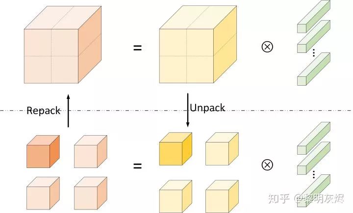
Figure 7: Steps of Spatial Packing Computation

It is worth noting that for convenience, the description above ignores the issue of Padding. In practice, when partitioning the input tensor into several small tensors in Step 1, in addition to copying the original data in the small blocks, it is also necessary to copy the boundary data of adjacent small tensors. Specifically, as shown in Figure 8, the shape of the small tensors obtained from spatial splitting is actually:

𝑁×(𝐻/ℎ+2(𝐾𝐻−1))×(𝑊/𝑤+(𝐾𝑊−1))×𝐶.(5)

Here, 2(𝐾𝐻−1) and 2(𝐾𝑊−1) follow the Padding rules. The rules are can be ignored; the rules are SAME, the Padding at one side of the source tensor boundary must be filled with zero; the Padding not at the source tensor boundary uses the values of neighboring tensors. This is evident when considering the principles of convolution calculations.

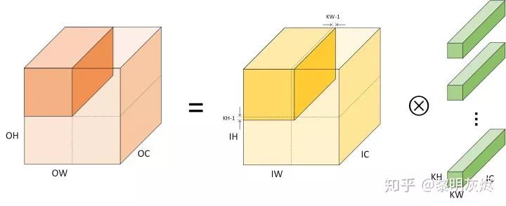
Figure 8: Details of Spatial Packing Algorithm Partitioning

The three example figures above all show the case of partitioning into 4 parts; in practical applications, they can be partitioned into many parts. For example, they can be divided into small tensors with a side length of 4 or 8, making it easier for the compiler to vectorize the computation operations. As the split tensors get smaller, their locality increases, but the negative effect is that more additional memory is consumed. This additional memory is due to Padding. When partitioned into ℎ∗𝑤h∗w parts, the memory consumed by Padding is:

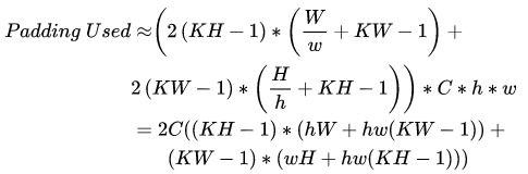
It can be seen that as the granularity of partitioning becomes smaller, the additional memory consumed increases. It is noteworthy that when partitioning to the finest granularity, that is, partitioning in the spatial domain of shape 𝑁×𝐻×𝑊×𝑂𝐶 into 𝐻∗𝑊 parts, spatial packing degenerates into the Im2col method. At this point, the convolution at one element is equivalent to the dot product when calculating one output element in matrix multiplication.

When only performing spatial partitioning, the partitioning is independent of the convolution kernel. However, if partitioning in the output channel dimension, the convolution kernel can also be correspondingly partitioned. Partitioning in the channel dimension is equivalent to simple stacking after fixing spatial partitioning, which does not affect memory consumption but will affect locality. Finding suitable partitioning methods for convolutions of different scales is not an easy task. Like many problems in the field of computer science, this problem can also be automated; for example, AutoTVM can find better partitioning methods in such cases.

• AutoTVM Link: https://arxiv.org/abs/1805.08166

Winograd Optimization Algorithm

The two algorithms introduced in the previous sections, Im2col, organize three-dimensional tensors into matrices and then call GEMM computing libraries, which largely utilize optimizations based on memory locality; the spatial packing optimization method is itself an optimization method that utilizes locality. This section introduces the Winograd optimization algorithm, which is an application of the matrix multiplication optimization method known as the Coppersmith–Winograd algorithm, based on algorithm analysis.

This part has too many formulas, making it inconvenient to format. If interested, please refer to the original text or other related literature.

Reference Original Text Link: https://jackwish.net/convolution-neural-networks-optimization.html

Indirect Convolution Optimization Algorithm

Marat Dukhan introduced the Indirect Convolution Algorithm in QNNPACK (Quantized Neural Network PACKage), which seems to be the fastest among all publicly available methods so far (as of mid-2019). Recently, the author published a related article to introduce the main ideas behind it.

Although the implementation of this algorithm in QNNPACK is mainly used for quantized neural networks (other quantization optimization schemes in the industry are relatively traditional, such as TensorFlow Lite using the Im2col optimization algorithm, Tencent’s NCNN using the Winograd optimization algorithm; OpenAI’s Tengine using the Im2col optimization algorithm), it is a similar design of optimization algorithms.

At the time of writing this article, the design of the article has not been publicly disclosed, and understanding many details of the algorithm design is best done in conjunction with the code.My QNNPACK fork contains an explained branch, which includes comments on some parts of the code for reference.

• QNNPACK Link: https://github.com/pytorch/QNNPACK

• TensorFlow Lite using the Im2col optimization algorithm Link: https://github.com/tensorflow/tensorflow/blob/v2.0.0-beta1/tensorflow/lite/kernels/internal/optimized/integer_ops/conv.h

• NCNN using the Winograd optimization algorithm Link: https://github.com/Tencent/ncnn/blob/20190611/src/layer/arm/convolution_3x3_int8.h

• Tengine using the Im2col optimization algorithm Link: https://github.com/OAID/Tengine/blob/v1.3.2/executor/operator/arm64/conv/conv_2d_fast.cpp

• My QNNPACK fork Link: https://github.com/jackwish/qnnpack

Computational Workflow

The effective operation of the Indirect Convolution Algorithm relies on a key premise—the memory address of the input tensor remains unchanged during continuous network operation. This characteristic is relatively easy to satisfy; even if the address really needs to change, it can be copied to a fixed memory area.

Figure 9: Workflow of the Indirect Convolution Algorithm

Figure 9 shows the detailed process of the workflow of the Indirect Convolution Algorithm. The leftmost part indicates that multiple inputs use the same input buffer (Input Buffer). The Indirect Convolution Algorithm will construct an “Indirect Buffer” based on this input buffer, which is the core of the Indirect Convolution Algorithm. As shown on the right side of the figure, during network operation, each computation produces an output of size 𝑀×𝑁, where 𝑀 is the vectorized scale considering 𝑂𝐻×𝑂𝑊 as one-dimensional. Generally, 𝑀×𝑁 is 4×4, 8×8, or 4×8. When calculating an output of size 𝑀×𝑁, the corresponding input is taken from the indirect buffer and the weights are retrieved to calculate the result. The calculation process is equivalent to calculating 𝑀×𝐾 and 𝐾×𝑁 matrix multiplication.

In implementation, the execution process of the software is divided into two parts:

1. Preparation phase: load the model, configure the input buffer; rearrange weights to make their memory layout suitable for subsequent calculations;

2. Execution phase: for each input, run ⌈𝑂𝐻∗𝑂𝑊/𝑀⌉∗⌈𝑂𝐶/𝑁⌉ core loops, calculating an output of size 𝑀×𝑁 each time using the GEMM method.

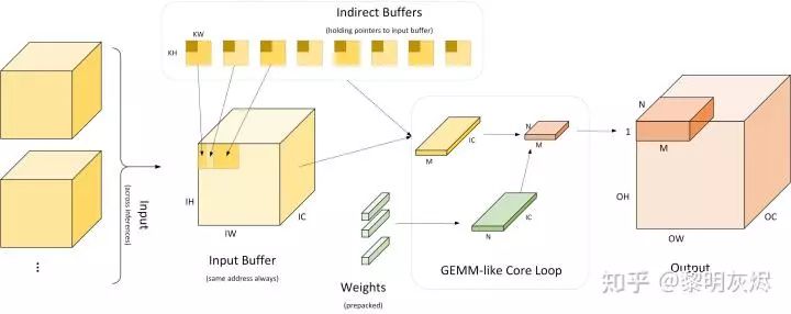
Figure 10: Indirect Buffer

As discussed in the relevant sections, the Im2col optimization algorithm has two problems: first, it occupies a large amount of additional memory; second, it requires extra data copying of the input. How can these two points be resolved? The indirect convolution algorithm provides the answer: the Indirect Buffer, as shown in the right half of Figure 10.

Figure 10 contrasts the conventional Im2col optimization algorithm with the indirect convolution optimization algorithm. As introduced in the relevant sections, the Im2col optimization algorithm first copies the input into a matrix, as indicated by the arrows related to Input in Figure 10, and then performs matrix multiplication. The indirect convolution optimization algorithm uses indirect buffers to store pointers to the input (which is also the reason why the indirect convolution optimization algorithm requires the input memory address to be fixed). During operation, the corresponding inputs are retrieved based on these pointers, and the weights are taken out to calculate the results. The calculation process is equivalent to the matrix multiplication of 𝑀×𝐾 and 𝐾×𝑁.

Layout of Indirect Buffer

The indirect buffer can be understood as a set of buffers of convolution kernel size, totaling 𝑂𝐻×𝑂𝑊, with each buffer sized 𝐾𝐻×𝐾𝑊—each buffer corresponds to the address of the input needed for a certain output. Each time an output at a spatial position is calculated, one indirect buffer is used; outputs at the same spatial position but different channels use the same indirect buffer, with each pointer in the buffer indexing the 𝐼𝐶 elements in the input. As the output moves, different indirect buffers are selected to obtain the corresponding input addresses. There is no need to calculate the input addresses based on the coordinates of the output target; this is equivalent to pre-calculating the addresses.

Figure 11 illustrates how the indirect buffer is used when 𝑀×𝑁 is 4, and both 𝐾𝐻 and 𝐾𝑊 are 3. The term local indirect buffer indicates that the focus is currently on the core calculation process of computing 𝑀×𝑁.

When calculating an output of size 𝑀×𝑁, the input used corresponds to the area covered by the convolution kernel sliding over the input at the corresponding position, leading to an input size of (𝐾𝐻)×(𝑀+2(𝐾𝑊−1))×𝐼𝐶. In the indirect convolution algorithm, these input memories are indexed by pointers in the 𝑀 indirect buffers, totaling 𝑀×𝐾𝐻×𝐾𝑊. Figure 11 marks the relationship between the input space position in the upper left corner and the corresponding input buffers. It can be seen that the A, B, C, and D input buffers here, the addresses pointed to by two adjacent buffers have (𝐾𝑊−𝑆𝑡𝑟𝑖𝑑𝑒)/𝐾𝑊, which is 2/3, and the coordinates of the pointers in each buffer are also marked.

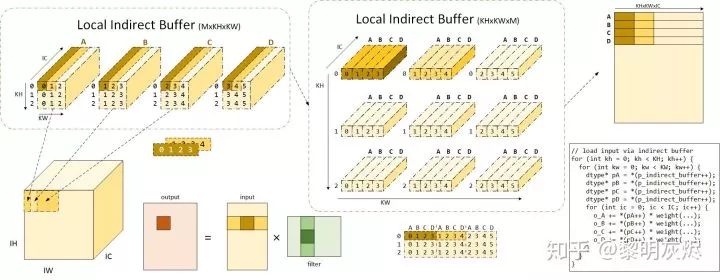
Figure 11: Detailed Explanation of the Indirect Buffer

The arrangement of the planar buffer is not the final layout; in fact, these pointers will be processed into the indirect buffer structure shown in the middle of Figure 11. By scattering the pointers in each buffer in the upper left, we can obtain 𝐾𝐻×𝐾𝑊 pointers. By collecting the pointers in A, B, C, and D buffers at different spatial positions together, we can achieve the buffer arrangement in the upper part of the figure as 𝐾𝐻×𝐾𝑊×𝑀. It can be seen that the pointers in the A, B, C, and D buffers at the same spatial position are organized together. The upper part of the figure shows the visual effect, while the lower part is the actual organization of the indirect buffer. The brown and dark yellow colors in the figure correspond to the same input memory or pointer. It is worth noting that in the legend, when Stride is 1, if Stride is not 1, the coordinates of A, B, C, and D at the same spatial position (corresponding to the coordinates in the input) may not be continuous, and the adjacent spatial positions differ by a Stride size.

Using Indirect Buffers for Computation

We have understood the organization of indirect buffers and how their pointers correspond to input memory addresses. Now, let’s explore how to use these buffers in the computation process.

Similar to the previous section, the discussion in this section generally focuses on computing outputs of size 𝑀×𝑁, where these outputs require 𝑀 inputs of size 𝐾𝐻×𝐾𝑊, with data reuse involved. Now, reviewing the Im2col algorithm (as shown in the lower left part of Figure 11), when running vectorized calculations for 𝑀×𝑁 matrix multiplication, each time retrieving inputs of size 𝑀×𝑆 and weights of size 𝑆×𝑁, we perform matrix multiplication on that block to obtain the corresponding partial sum and result. Here, 𝑆 is the stepping factor for vectorized calculations in the 𝐾 dimension.

The reason convolution can use the Im2col optimization algorithm is fundamentally because its decomposed calculation process, ignoring memory reuse, is equivalent to matrix multiplication. The indirect buffer allows simulating memory access to the input through pointers. During the actual computation of the output of size 𝑀×𝑁, the micro kernel will scan the input with 𝑀 pointers. Each of the 𝑀 pointers retrieves 𝑀 addresses from the indirect buffer structure in the lower part of Figure 11, corresponding to the memory of size 𝑀×𝐼𝐶 in the input, as shown in the upper right corner layout. In this stepping, the operation still runs in the form of 𝑀×𝑆, where 𝑆 moves in the 𝐼𝐶 dimension. After scanning this part of the input, these 𝑀 pointers fetch the corresponding pointers from the indirect buffer and continue to the next traversal of the 𝑀×𝐼𝐶 input memory, calculating the output partial sum of size 1/(𝐾𝐻∗𝐾𝑊) each time. After this process runs 𝐾𝐻×𝐾𝑊 times, we obtain the output of size 𝑀×𝑁. The pseudocode in the lower right corner of Figure 11 corresponds to this process. Since the indirect buffer has already been organized into a specific shape, each time updating the 𝑀 pointers only requires fetching from the indirect buffer pointers (the p_indirect_buffer in the pseudocode in the figure).

This process is logically difficult to understand; here are some additional explanations. When the above 𝑀 pointers continuously move to scan memory, they are effectively scanning the matrix after the input has been unfolded by Im2col. The specific nature of the input buffer is that it transforms the scanning of a two-dimensional matrix into scanning a three-dimensional tensor. The scanning process of the input corresponds to the visualization of the input in the upper part of Figure 11; relating the upper left and lower left corresponding input relationships, it is not difficult to find that each time it scans a block of size 𝑀×𝐼𝐶 in the input. It is noteworthy that the 𝑀×𝐼𝐶 here consists of 𝑀 tensors of size 1×𝐼𝐶, with a stride size of 𝑆𝑡𝑟𝑖𝑑𝑒 between them.

Thus, by running this computing core ⌈𝑂𝐻∗𝑂𝑊/𝑀⌉∗⌈𝑂𝐶/𝑁⌉ times, we can obtain all outputs.

The indirect convolution optimization algorithm addresses three issues in convolution calculations: first, the spatial vectorization issue; second, the complexity of address calculations; third, the memory copy problem. Generally, convolution calculations require zero-padding on the input (for cases where 𝐾𝐻×𝐾𝑊 is not 1×1); traditional methods usually incur memory copies during this process. However, the indirect buffers in the indirect convolution optimization algorithm cleverly resolve this issue through indirect pointers. In constructing the indirect buffer, an additional 1×𝐼𝐶 memory buffer is created, filled with zero values. For spatial positions requiring zero-padding, the corresponding indirect pointers are directed to this buffer, meaning that subsequent calculations are equivalent to having already zero-padded. For example, in Figure 11, the upper left corner of A corresponds to the input spatial position (0,0); when zero-padding is needed, this position must be zero, and at this point, it suffices to modify the address in the indirect buffer.

Discussion, Summary, and Outlook

So far, this article has explored some published or open-source optimization methods for convolutional neural networks. These optimization methods have, to varying degrees, promoted the application of deep learning technology in cloud or mobile scenarios, aiding our daily lives. For instance, the recent garbage classification problem troubling the people of Shanghai and even all of China can also be addressed using deep learning methods to help people understand how to classify.

• Using deep learning methods to help people understand how to classify Link: https://news.mydrivers.com/1/633/633858.htm

From the concentrated optimization methods in this article, it can be seen that the optimization algorithms for convolutional neural networks can still encompass methods based on algorithm analysis and methods based on software optimization. In fact, in modern computer systems, software optimization methods, especially those based on computer storage hierarchy, are more important as they are easier to exploit and apply. On the other hand, the newly added dedicated instructions in modern computers can already erase the time differences of different computations. In such scenarios, combining algorithm analysis methods with software optimization methods might yield better optimization results.

Finally, the optimization methods discussed in this article are fundamentally general methods, and with the development of neural network processors (such as Cambricon MLU, Google TPU) and the expansion of other general-purpose computing processors (such as instructions related to dot products: Nvidia GPU DP4A, Intel AVX-512 VNNI, ARM SDOT/UDOT ), the optimization of deep learning may still deserve continued investment of resources.

• Cambricon MLU Link: https://www.jiqizhixin.com/articles/2019-06-20-12

• Nvidia GPU DP4A Link: https://devblogs.nvidia.com/mixed-precision-programming-cuda-8/

• Intel AVX-512 VNN Link: https://devblogs.nvidia.com/mixed-precision-programming-cuda-8/

This article references the following materials (including but not limited to):

• QNNPACK （ Link: https://github.com/pytorch/QNNPACK ）

• Convolution in Caffe （ Link: https://github.com/Yangqing/caffe/wiki/Convolution-in-Caffe:-a-memo ）

• TensorFlow

• Wikipedia

• Fast Algorithms for Convolutional Neural Networks （ Link: https://github.com/Tencent/ncnn ）

• NCNN（ Link: https://github.com/OAID/Tengine ）

• Tengine （ Link: https://jackwish.net/neural-network-quantization-introduction-chn.html ）

• Introduction to Neural Network Quantization （ Link: https://jackwish.net/neural-network-quantization-introduction-chn.html ）

• General Matrix Multiplication (GEMM) Optimization Algorithm （ Link: https://jackwish.net/gemm-optimization.html ）

• The Indirect Convolution Algorithm

Download 1: OpenCV-Contrib Extension Module Chinese Tutorial

Reply "Extension Module Chinese Tutorial" in the backend of the "Beginner Learning Vision" public account to download the first OpenCV extension module tutorial in Chinese on the internet, covering installation of extension modules, SFM algorithms, stereo vision, target tracking, biological vision, super-resolution processing, and more than twenty chapters of content.

Download 2: 52 Lectures on Python Vision Practical Projects

Reply "Python Vision Practical Projects" in the backend of the "Beginner Learning Vision" public account to download 31 visual practical projects, including image segmentation, mask detection, lane line detection, vehicle counting, eyeliner addition, license plate recognition, character recognition, emotion detection, text content extraction, facial recognition, etc., to help quickly learn computer vision.

Download 3: 20 Lectures on OpenCV Practical Projects

Reply "20 Lectures on OpenCV Practical Projects" in the backend of the "Beginner Learning Vision" public account to download 20 practical projects based on OpenCV.

Discussion Group

You are welcome to join the reader group of the public account to communicate with peers. Currently, there are WeChat groups on SLAM, 3D vision, sensors, autonomous driving, computational photography, detection, segmentation, recognition, medical imaging, GAN, algorithm competitions, etc. (these will gradually be subdivided in the future). Please scan the WeChat ID below to join the group, and note: "Nickname + School/Company + Research Direction", for example: "Zhang San + Shanghai Jiao Tong University + Visual SLAM". Please follow the format; otherwise, you will not be approved. After successful addition, you will be invited to join the relevant WeChat group based on your research direction. Please do not send advertisements in the group; otherwise, you will be removed from the group. Thank you for your understanding~