Author: Ye Hu

Editor: Tian Xu

Recently, deep CNN networks like ResNet and DenseNet have significantly improved the accuracy of image classification. However, in addition to accuracy, computational complexity is also an important metric for CNN networks. Overly complex networks may be very slow, and specific scenarios, such as autonomous driving, require low latency. Moreover, mobile devices need small models that are both accurate and fast. To meet these demands, lightweight CNN networks such as MobileNet and ShuffleNet have been proposed, which achieve a good balance between speed and accuracy. Today, we will discuss ShuffleNetv2, the upgraded version of ShuffleNet recently proposed by Megvii, which was included in ECCV2018. Under the same complexity, ShuffleNetv2 is more accurate than ShuffleNet and MobileNetv2.

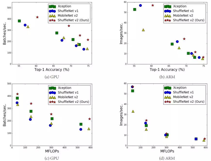
Figure 1: Comparison of complexity, speed, and accuracy of ShuffleNetv2 with other algorithms on different platforms

Design Philosophy

A common metric for measuring model complexity is FLOPs, which specifically refers to the number of multiply-add operations. However, this is an indirect metric because it does not fully correspond to speed. As seen in (c) and (d) of Figure 1, two models with the same FLOPs can exhibit different speeds. This inconsistency is primarily attributed to two reasons. First, factors affecting speed are not limited to FLOPs, such as memory access cost (MAC), which cannot be ignored and can be a bottleneck for GPUs. Additionally, the degree of parallelism of the model also affects speed; models with higher parallelism are relatively faster. Another reason is that the running speed of models varies across different platforms, such as GPU and ARM, and using different libraries can also have an impact.

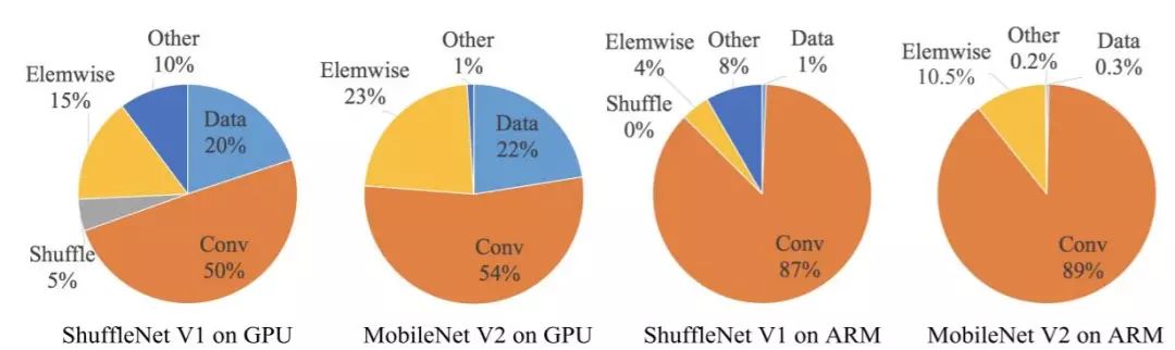
Figure 2: Breakdown of running time of different models

Accordingly, the author studied the running times of ShuffleNetv1 and MobileNetv2 on specific platforms and derived four practical guidelines through theoretical and experimental analysis:

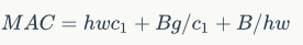
(G1) Minimize memory access for equal channel sizes. Lightweight CNN networks often use depthwise separable convolutions, where pointwise convolution (1×1 convolution) has the highest complexity. Assuming the number of input and output feature channels are and , and the spatial size of the feature map is , then the FLOPs of the 1×1 convolution is . The corresponding MAC (assuming sufficient memory) is 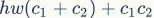. According to the mean inequality, when fixed, the MAC has a lower limit (let ):

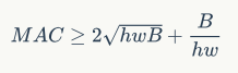
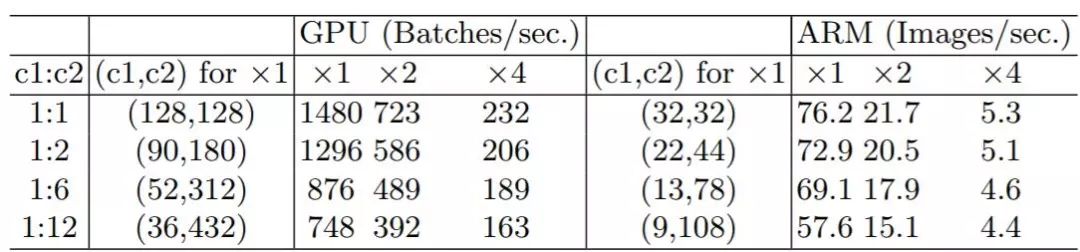
Only when is the MAC minimized. This theoretical analysis is also confirmed by experiments, as shown in Table 1, where the speed is faster when the channel ratio is 1:1.

Table 1: Experimental validation of G1

(G2) Overuse of group convolutions increases MAC. Group convolution is a commonly used design component because it can reduce complexity without losing model capacity. However, it has been found that too many groups can increase MAC. For group convolution, the FLOPs is 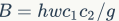, while the corresponding MAC is 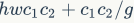. If the input and B are fixed, then the MAC is:

It can be seen that as g increases, the MAC also increases. This has also been confirmed by experiments, so it is wise not to use too large a group for group convolutions.

(G3) Network fragmentation reduces parallelism. Some networks like Inception and NASNET-A generated by Auto ML tend to adopt a “multi-path” structure, which contains many different small convolutions or pooling operations, easily causing network fragmentation and reducing model parallelism, resulting in slower speeds, as confirmed by experiments.

(G4) Element-wise operations cannot be ignored. For element-wise operators like ReLU and Add, although their FLOPs are small, they require significant MAC. Experiments have shown that removing ReLU and shortcut from the residual units in ResNet can lead to a 20% speed improvement.

The above four guidelines can be summarized as follows:

• Balance the input and output channel sizes with 1×1 convolutions;

• Use group convolutions cautiously and pay attention to the number of groups;

• Avoid network fragmentation;

• Reduce element-wise operations.

Network Structure

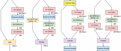
Based on the four guidelines mentioned earlier, the author analyzed the shortcomings of ShuffleNetv1’s design and improved it to obtain ShuffleNetv2. The comparison of the two modules is shown in Figure 3:

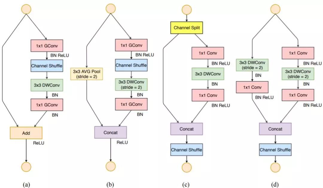
Figure 3: Structural comparison between the two versions of ShuffleNet

In ShuffleNetv1’s module, 1×1 group convolutions are used extensively, which violates the G2 principle. Additionally, v1 adopted a bottleneck layer similar to ResNet, where the input and output channel numbers are different, violating the G1 principle. At the same time, using too many groups also violates the G3 principle. There are a large number of element-wise Add operations in the shortcut connections, which violates the G4 principle.

To address the shortcomings of v1, the v2 version introduces a new operation: channel split. Specifically, the input feature map is first split into two branches along the channel dimension: with channel numbers and . In practice, . The left branch performs equal mapping, while the right branch contains three consecutive convolutions, and the input and output channels are the same, which complies with G1. Moreover, the two 1×1 convolutions are no longer group convolutions, which complies with G2. Additionally, the two branches are effectively divided into two groups. The outputs of the two branches are no longer added element-wise but concatenated, followed by a channel shuffle operation to ensure information exchange between the two branches. In fact, the concatenation and channel shuffle can be combined into a single element-wise operation with the next module’s channel split, which complies with principle G4.

For the down-sampling module, there is no channel split; instead, each branch directly copies an input, and each branch has stride=2 down-sampling. Finally, after concatenation, the spatial size of the feature map is halved, but the number of channels doubles.

The overall structure of ShuffleNetv2 is shown in Table 2, which is essentially similar to v1, where the channel number for each block is set, such as 0.5x, 1x, allowing adjustment of the model’s complexity.

Table 2: Overall structure of ShuffleNetv2

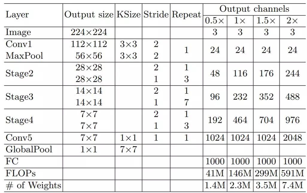
It is worth noting that v2 adds a conv5 convolution before global pooling, which is a distinction from v1. The final model’s classification performance on ImageNet is shown in Table 3:

Table 3: ShuffleNetv2 classification performance on ImageNet

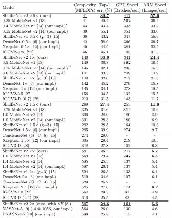
As can be seen, under the same conditions, ShuffleNetv2 is slightly faster than other models and also has slightly better accuracy. At the same time, the author also designed a larger ShuffleNetv2 network, which remains competitive compared to ResNet structures.

To some extent, ShuffleNetv2 draws from the DenseNet network, changing the shortcut structure from Add to Concat, achieving feature reuse. However, unlike DenseNet, v2 does not concatenate densely but applies channel shuffle after concatenation to mix features, which may be an important reason why v2 is both fast and effective.

Implementation on TensorFlow

Currently, there is no official open-source implementation of ShuffleNetv2. Here, we refer to a reproduction in tensorpack (where the Top1 accuracy is close to that in the paper) and provide an implementation of v2 in TensorFlow. We use tf.keras.Model in TensorFlow to implement ShuffleNetv2.

First, we define the most basic unit in the network: Conv2D->BN->ReLU and DepthwiseConv2D->BN:

class Conv2D_BN_ReLU(tf.keras.Model):
    """Conv2D -> BN -> ReLU"""
    def __init__(self, channel, kernel_size=1, stride=1):
        super(Conv2D_BN_ReLU, self).__init__()

        self.conv = Conv2D(channel, kernel_size, strides=stride,
                            padding="SAME", use_bias=False)
        self.bn = BatchNormalization(axis=-1, momentum=0.9, epsilon=1e-5)
        self.relu = Activation("relu")

    def call(self, inputs, training=True):
        x = self.conv(inputs)
        x = self.bn(x, training=training)
        x = self.relu(x)
        return x

class DepthwiseConv2D_BN(tf.keras.Model):
    """DepthwiseConv2D -> BN"""
    def __init__(self, kernel_size=3, stride=1):
        super(DepthwiseConv2D_BN, self).__init__()

        self.dconv = DepthwiseConv2D(kernel_size, strides=stride,
                                     depth_multiplier=1,
                                     padding="SAME", use_bias=False)
        self.bn = BatchNormalization(axis=-1, momentum=0.9, epsilon=1e-5)

    def call(self, inputs, training=True):
        x = self.dconv(inputs)
        x = self.bn(x, training=training)

For channel shuffle, it can be easily achieved through reshape operations:

def channle_shuffle(inputs, group):
    """Shuffle the channel
    Args:
        inputs: 4D Tensor
        group: int, number of groups
    Returns:
        Shuffled 4D Tensor
    """
    in_shape = inputs.get_shape().as_list()
    h, w, in_channel = in_shape[1:]
    assert in_channel % group == 0
    l = tf.reshape(inputs, [-1, h, w, in_channel // group, group])
    l = tf.transpose(l, [0, 1, 2, 4, 3])
    l = tf.reshape(l, [-1, h, w, in_channel])

    return l

class ShufflenetUnit1(tf.keras.Model):
    def __init__(self, out_channel):
        """The unit of shufflenetv2 for stride=1
        Args:
            out_channel: int, number of channels
        """
        super(ShufflenetUnit1, self).__init__()

        assert out_channel % 2 == 0
        self.out_channel = out_channel

        self.conv1_bn_relu = Conv2D_BN_ReLU(out_channel // 2, 1, 1)
        self.dconv_bn = DepthwiseConv2D_BN(3, 1)
        self.conv2_bn_relu = Conv2D_BN_ReLU(out_channel // 2, 1, 1)

    def call(self, inputs, training=False):
        # split the channel
        shortcut, x = tf.split(inputs, 2, axis=3)

        x = self.conv1_bn_relu(x, training=training)
        x = self.dconv_bn(x, training=training)
        x = self.conv2_bn_relu(x, training=training)

        x = tf.concat([shortcut, x], axis=3)
        x = channle_shuffle(x, 2)
        return x

class ShufflenetUnit2(tf.keras.Model):
    """The unit of shufflenetv2 for stride=2"""
    def __init__(self, in_channel, out_channel):
        super(ShufflenetUnit2, self).__init__()

        assert out_channel % 2 == 0
        self.in_channel = in_channel
        self.out_channel = out_channel

        self.conv1_bn_relu = Conv2D_BN_ReLU(out_channel // 2, 1, 1)
        self.dconv_bn = DepthwiseConv2D_BN(3, 2)
        self.conv2_bn_relu = Conv2D_BN_ReLU(out_channel - in_channel, 1, 1)

        # for shortcut
        self.shortcut_dconv_bn = DepthwiseConv2D_BN(3, 2)
        self.shortcut_conv_bn_relu = Conv2D_BN_ReLU(in_channel, 1, 1)

    def call(self, inputs, training=False):
        shortcut, x = inputs, inputs

        x = self.conv1_bn_relu(x, training=training)
        x = self.dconv_bn(x, training=training)
        x = self.conv2_bn_relu(x, training=training)

        shortcut = self.shortcut_dconv_bn(shortcut, training=training)
        shortcut = self.shortcut_conv_bn_relu(shortcut, training=training)

        x = tf.concat([shortcut, x], axis=3)
        x = channle_shuffle(x, 2)
        return x