Say Goodbye to Vlookup: Introducing GETPIVOTDATA Function!

The most commonly used lookup function in Excel is the Vlookup function. If you encounter more complex situations, you can use the Lookup function, but there is one case where both of these functions can only stand by, which is the lookup in a Pivot Table.

Sales Detail Table

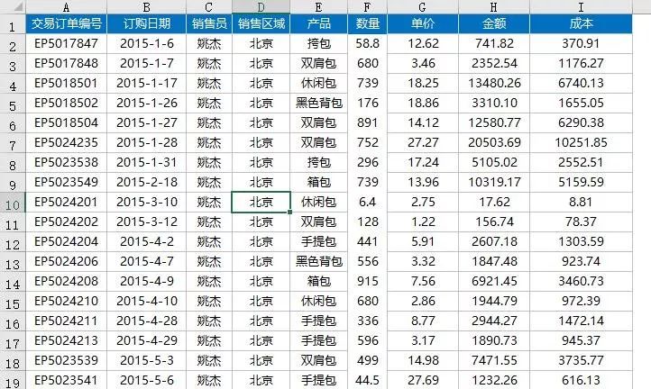
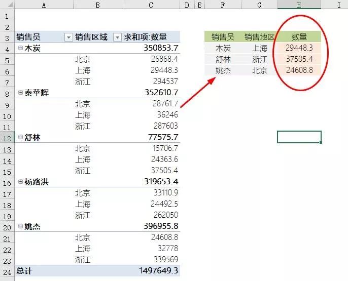
After summarizing using the Pivot Table (A:C columns), you need to extract the corresponding data from the left Pivot Table based on columns F and G in the right table below, as shown in column H.

There is a function in Excel specifically designed for Pivot Tables, which is the

GETPIVOTDATA function

It can extract data from the Pivot Table based on conditions, and its usage is quite simple:

=GETPIVOTDATA(Extracted Column,Any Cell in the Pivot Table,Column 1,Condition 1,Column 2,Condition 2,…Column N,Condition N)

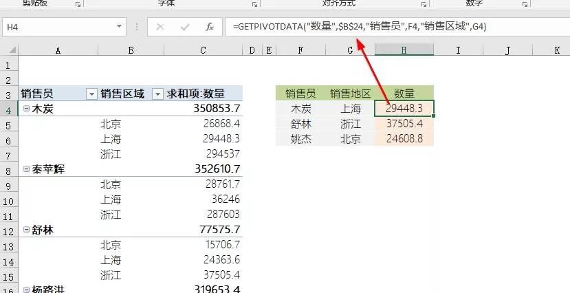
The extraction formula in this example is:

Formula in H4

=GETPIVOTDATA(“Quantity”,$B$24,“Salesperson”,F4,“Sales Region”,G4)

Formula Explanation:

• Quantity: The result column to extract

• $B$24: Any cell in the Pivot Table

• “Salesperson”,F4: The salesperson is the value of cell F4

• “Sales Region”,G4: The sales region is the value of cell G4

In actual work, the results summarized by the Pivot Table are sometimes just used as transitional data, for example, when you need to verify the results after summarizing two tables. In this case, you first summarize with the Pivot Table, and then use GETPIVOTDATA to extract data for verification.

Source: Excel Elite Training