
In Excel, the most commonly used lookup function is the Vlookup function. If you encounter more complex situations, you can use the Lookup function. However, there is a case where both of these functions can only stand by, which is the lookup for PivotTables.
Sales Detail Table
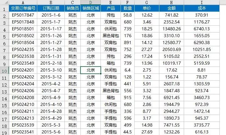
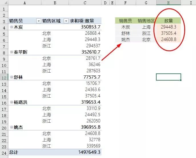
After summarizing using the PivotTable (columns A:C), you need to extract the corresponding data from the left PivotTable into the right table based on columns F and G, as shown in column H.
Excel has a function specifically designed for PivotTables, which is
GETPIVOTDATA function
This function can extract data from a PivotTable based on conditions, and its usage is quite simple:
=GETPIVOTDATA(extracted column,any cell in the PivotTable,column 1,condition 1,column 2,condition 2,…column N,condition N)
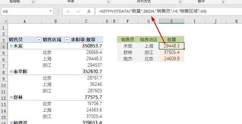
The extraction formula in this example is:
Formula in H4
=GETPIVOTDATA(“Quantity”,$B$24,“Salesperson”,F4,“Sales Region”,G4)
Formula Explanation:
-
Quantity: the result column to extract
-
$B$24: any cell in the PivotTable
-
“Salesperson”,F4: the salesperson is the value in cell F4
-
“Sales Region”,G4: the sales region is the value in cell G4
Lan Se said: In actual work, the results summarized by the PivotTable are sometimes used as transitional data, for example, to verify the results of two summarized tables. In this case, first use the PivotTable to summarize, and then use GETPIVOTDATA to extract data for verification.
If you are a new student, long press the QR code below – identify the QR code in the image – follow us, and you can learn Excel with Lan Se every day.