SAC Algorithm in Deep Reinforcement Learning: Mathematical Principles, Network Architecture, and PyTorch Implementation

Source: DeepHub IMBA

This article is approximately 3600 words long, and it is recommended to read it in 7 minutes.
This article will systematically elaborate on the technical details of the SAC algorithm.

Deep reinforcement learning is one of the most challenging research directions in the field of artificial intelligence, with its design concept originating from the mechanism of biological learning systems optimizing decisions based on experience. Among the many deep reinforcement learning algorithms, the Soft Actor-Critic (SAC) algorithm has attracted much attention due to its excellent performance in sample efficiency, exploration effectiveness, and training stability.

Traditional deep reinforcement learning algorithms often face challenges in exploration-exploitation trade-offs and training stability. The SAC algorithm effectively addresses these issues by introducing a maximum entropy reinforcement learning framework, which automatically adjusts the level of exploration during the policy optimization process. Its core innovation lies in maximizing entropy as an additional objective for policy optimization, maintaining policy diversity while ensuring convergence.

This article will systematically elaborate on the technical details of the SAC algorithm, mainly including:

1. Mathematical principles of the SAC algorithm based on the maximum entropy framework

2. Specific architectural design of the actor and critic networks

3. Detailed implementation plan based on PyTorch

4. Key technical points for network training

The SAC algorithm adopts an actor-critic architecture, where the actor network is responsible for generating action policies, and the critic network evaluates the action values. Through the collaborative optimization of the two networks, the policy is gradually improved. Throughout the training process, the actor network aims to maximize the Q-values predicted by the critic network while maintaining a moderate level of policy exploration; the critic network continuously optimizes the accuracy of its Q-value estimates.

Next, we will start with the mathematical principles of the actor network and analyze the various technical components of the SAC algorithm in detail:

Actor (Policy) Network

The actor is a policy network determined by parameters φ, represented as:

This is a stochastic policy based on state outputs. It uses a neural network to estimate the mean and log standard deviation, thus obtaining the distribution of actions and their log probabilities given a state. The log probabilities are used for entropy regularization, meaning that the objective function includes a term aimed at maximizing the breadth of the probability distribution (entropy) to promote the agent’s exploratory behavior. Details on entropy regularization will be elaborated later. The architecture of the actor network is shown in the figure below:

The mean μ(s) and log σ(s) are used for action sampling:

Where N represents a normal distribution. However, this operation has a gradient non-differentiability issue, which needs to be solved by the reparameterization trick.

Here d represents the action space dimension, and each component ε_i is sampled from a standard normal distribution (mean 0, standard deviation 1). Applying the reparameterization trick:

This resolves the gradient truncation issue. Next, the activation function is used to transform x_t into normalized actions:

This transformation ensures that actions are constrained within the [-1,1] interval.

Action Log Probability Calculation

After calculating the action, we can compute the reward and expected return. The actor’s loss function also includes an entropy regularization term to maximize the breadth of the distribution. When calculating the log probability of the sampled action 𝑎t, it is more convenient to analyze starting from the pre-tanh transformation x_t.

Since x_t comes from the Gaussian distribution of mean μ(s) and standard deviation σ(s), its probability density function (PDF) is:

Where the distribution of each independent component x_t,i is:

Taking the logarithm of both sides simplifies the PDF:

To convert it to log(π_ϕ), we need to consider the tanh transformation from x_t to a_t, which can be achieved using the differential chain rule:

The derivation of this relationship is based on the principle of probability conservation: the probabilities of two variables within a given interval must be equal:

Where a_i = tanh(x_i). Reducing the interval to infinitesimal dx and da:

The derivative form of tanh is:

Substituting gives:

We can finally obtain the complete expression:

Thus, the derivation of the actor part is completed; here we have both actions and log probabilities, which allows us to calculate the loss function. Below is the PyTorch implementation of these mathematical expressions:

 import gymnasium as gym   from src.utils.logger import logger   from src.models.callback import PolicyGradientLossCallback   from pydantic import Field, BaseModel, ConfigDict   from typing import Dict, List   import numpy as np   import os   from pathlib import Path   import torch   import torch.nn as nn   import torch.optim as optim   import torch.nn.functional as F   from torch.distributions import Normal  
 '''Actor network: estimates mean and log standard deviation for entropy regularization calculation'''  class Actor(nn.Module):       def __init__(self,state_dim,action_dim):           super(Actor,self).__init__()  
         self.net = nn.Sequential(               nn.Linear(state_dim, 100),               nn.ReLU(),               nn.Linear(100,100),               nn.ReLU()           )           self.mean_linear = nn.Linear(100, action_dim)           self.log_std_linear = nn.Linear(100, action_dim)  
     def forward(self, state):           x = self.net(state)           mean = self.mean_linear(x)           log_std =self.log_std_linear(x)           log_std = torch.clamp(log_std, min=-20, max=2)           return mean, log_std  
     def sample(self, state):           mean, log_std = self.forward(state)           std = log_std.exp()           normal = Normal(mean, std)           x_t = normal.rsample() # Reparameterization trick           y_t = torch.tanh(x_t)           action = y_t           log_prob = normal.log_prob(x_t)           log_prob -= torch.log(1-y_t.pow(2)+1e-6)           log_prob = log_prob.sum(dim=1, keepdim =True)  
         return action, log_prob

Before discussing the definition of the loss function and the training process of the actor network, we need to introduce the mathematical principles of the critic network.

Critic Network

The core function of the critic network is to estimate the expected return (Q-value) of state-action pairs. These estimates provide guidance to the actor network during training. The critic network adopts a double network structure, providing two independent estimates of expected returns and selecting the smaller value as the final estimate. This design effectively avoids overestimation bias and enhances training stability. Its structure is shown in the figure below:

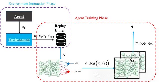
It should be noted that the schematic diagram at this time is a simplified version, mainly for understanding the basic roles of the actor and critic networks, without considering the details of training stability. Additionally, the term “agent” actually refers to the actor and critic networks collectively rather than as independent entities; the separate representation in the figure is just to clearly show the structure. Assume that the critic network does not need to be trained at this moment, as this allows us to focus on how to use the Q-values estimated by the critic network to train the actor network. The loss function expression for the actor network is:

A more common form is:

Where ρD represents the state distribution. The loss function is obtained by integrating the entropy terms over all action and state spaces with the Q-values. However, in practical applications, the complete state distribution cannot be directly obtained, so ρD is actually based on the empirical state distribution of replay buffer samples, expecting it to well represent the overall state distribution characteristics.

Based on this loss function, the actor network can be trained through backpropagation. Below is the PyTorch implementation of the critic network:

 '''Critic network: defining q1 and q2'''   class Critic(nn.Module):       def __init__(self, state_dim, action_dim):           super(Critic, self).__init__()  
         # Q1 network architecture           self.q1_net = nn.Sequential(               nn.Linear(state_dim + action_dim, 256),               nn.ReLU(),               nn.Linear(256, 256),               nn.ReLU(),               nn.Linear(256, 1),           )  
         # Q2 network architecture           self.q2_net = nn.Sequential(               nn.Linear(state_dim + action_dim, 256),               nn.ReLU(),               nn.Linear(256, 256),               nn.ReLU(),               nn.Linear(256, 1),           )  
     def forward(self, state, action):           sa = torch.cat([state, action], dim=1)           q1 = self.q1_net(sa)           q2 = self.q2_net(sa)           return q1, q2

The aforementioned content has not yet addressed the training mechanism of the critic network. Each data point sampled from the replay buffer contains [s_t, s_{t+1}, a_t, R]. For the Q-value of the state-action pair, we can obtain two different estimates.

The first method is to directly input a_t and s_t into the critic network:

The second method is based on the Bellman equation:

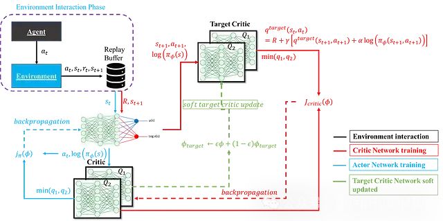
This method uses s_t+1, a_t+1, and the reward obtained from taking action a_t to re-estimate. Here, a target network is used instead of the critic network in the first method for estimation. The main purpose of using the target critic network is to address training instability. If the same critic network is used to generate Q-values for both the current state and the next state (used for target Q-values), this coupling can lead to inconsistent propagation of network updates at both ends of the target calculation, causing training instability. Therefore, an independent target network is introduced to provide stable estimates for the next state’s Q-values. The specific structure is shown in the figure below:

The loss function of the critic network is defined as:

Using this loss function, the critic network can be updated using backpropagation, while the target network adopts a soft update mechanism:

Where ε is a small constant used to limit the update magnitude of the target critic, thus maintaining training stability.

Complete Process

The above content has fully elaborated on the various components of the SAC agent. The following figure shows the complete structure and computational process of the SAC agent:

Below is a comprehensive implementation of the SAC agent that integrates the actor network, critic network, and their update mechanisms:

 '''SAC agent implementation: integrating actor network and critic network'''  class SACAgent:       def __init__(self, state_dim, action_dim, learning_rate, device):           self.device = device  
         self.actor = Actor(state_dim, action_dim).to(device)           self.actor_optimizer = optim.Adam(self.actor.parameters(), lr=learning_rate)  
         self.critic = Critic(state_dim, action_dim).to(device)           self.critic_optimizer = optim.Adam(self.critic.parameters(), lr=learning_rate)  
         # Target network initialization           self.critic_target = Critic(state_dim, action_dim).to(device)           self.critic_target.load_state_dict(self.critic.state_dict())  
         # Entropy temperature parameter           self.target_entropy = -action_dim            self.log_alpha = torch.zeros(1, requires_grad=True, device=device)           self.alpha_optimizer = optim.Adam([self.log_alpha], lr=learning_rate)  
     def select_action(self, state, evaluate=False):           state = torch.FloatTensor(state).to(self.device).unsqueeze(0)           if evaluate:               with torch.no_grad():                   mean, _ = self.actor(state)                   action = torch.tanh(mean)                   return action.cpu().numpy().flatten()           else:               with torch.no_grad():                   action, _ = self.actor.sample(state)                   return action.cpu().numpy().flatten()  
     def update(self, replay_buffer, batch_size=256, gamma=0.99, tau=0.005):           # Sample training data from experience replay           batch = replay_buffer.sample_batch(batch_size)           state = torch.FloatTensor(batch['state']).to(self.device)           action = torch.FloatTensor(batch['action']).to(self.device)           reward = torch.FloatTensor(batch['reward']).to(self.device)           next_state = torch.FloatTensor(batch['next_state']).to(self.device)           done = torch.FloatTensor(batch['done']).to(self.device)  
         # Critic network update           with torch.no_grad():               next_action, next_log_prob = self.actor.sample(next_state)               q1_next, q2_next = self.critic_target(next_state, next_action)               q_next = torch.min(q1_next, q2_next) - torch.exp(self.log_alpha) * next_log_prob               target_q = reward + (1 - done) * gamma * q_next  
         q1_current, q2_current = self.critic(state, action)           critic_loss = F.mse_loss(q1_current, target_q) + F.mse_loss(q2_current, target_q)  
         self.critic_optimizer.zero_grad()           critic_loss.backward()           self.critic_optimizer.step()  
         # Actor network update           action_new, log_prob = self.actor.sample(state)           q1_new, q2_new = self.critic(state, action_new)           q_new = torch.min(q1_new, q2_new)           actor_loss = (torch.exp(self.log_alpha) * log_prob - q_new).mean()  
         self.actor_optimizer.zero_grad()           actor_loss.backward()           self.actor_optimizer.step()  
         # Temperature parameter update           alpha_loss = -(self.log_alpha * (log_prob + self.target_entropy).detach()).mean()  
         self.alpha_optimizer.zero_grad()           alpha_loss.backward()           self.alpha_optimizer.step()  
         # Target network soft update           for param, target_param in zip(self.critic.parameters(), self.critic_target.parameters()):               target_param.data.copy_(tau * param.data + (1 - tau) * target_param.data

Conclusion

This article systematically elaborated on the mathematical foundations and implementation details of the SAC algorithm. Through an in-depth analysis of the actor and critic networks, we can see that the SAC algorithm has significant advantages in the following areas:

Theoretical Framework

• The theoretical foundation based on maximum entropy reinforcement learning ensures the convergence of the algorithm

• The double Q-network design effectively reduces overestimation bias in value function estimates

• The adaptive temperature parameter achieves a dynamic balance between exploration and exploitation

Implementation Features

• The reparameterization trick ensures the continuity of policy gradients

• The soft update mechanism enhances training stability

• The vectorized implementation based on PyTorch improves computational efficiency

Practical Value

• The algorithm performs excellently in continuous action spaces

• High sample efficiency makes it suitable for practical application scenarios

• The training process is stable, with relatively low difficulty in hyperparameter tuning

Future research can continue to deepen in the following directions:

• Exploring more efficient policy representations

• Studying the extension of the SAC algorithm in multi-agent scenarios

• Combining transfer learning to enhance the algorithm’s generalization ability

• Optimizing network architecture for large-scale state spaces

As a core research direction in artificial intelligence, reinforcement learning’s theoretical system and application scenarios are continuously evolving. A deep understanding of the mathematical principles and implementation details of the algorithm will help us grasp the essence of technology in this rapidly evolving field and develop more effective solutions.

Editor: Yu TengkaiProofreader: Liang Jincheng

About Us

Data Pie THU, as a public account focused on data science, is backed by the Big Data Research Center of Tsinghua University, sharing cutting-edge data science and big data technology innovation research dynamics, continuously disseminating data science knowledge, and striving to build a platform for gathering data talents and creating the strongest group of big data in China.

Sina Weibo: @Data Pie THU

WeChat Video Number: Data Pie THU

Today’s Headlines: Data Pie THU