This article lists some well-designed and practical “plugins” in CNN networks. A “plugin” does not change the main structure of the network, can be easily embedded into mainstream networks, and enhances the network’s feature extraction capabilities, achieving plug-and-play. There are many similar summary works in the field, all claiming to be plug-and-play and painless. However, based on my experience and collection, I found that many plugins are impractical, non-general, or even non-functional, hence this article.

First, my understanding is: since it is a “plugin”, it should add value, be easy to implement, and truly be plug-and-play. The “plugins” listed in this article can be seen in many SOTA networks. These are conscientious “plugins” worth promoting, truly capable of plug-and-play. In short, they are “plugins” that can work. Many “plugins” are introduced to enhance CNN capabilities, such as translation, rotation, scale transformation capabilities, multi-scale feature extraction capabilities, receptive field capabilities, spatial position perception capabilities, etc.

Shortlist: STN, ASPP, Non-local, SE, CBAM, DCNv1&v2, CoordConv, Ghost, BlurPool, RFB, ASFF

From Paper: Spatial Transformer Networks

Paper Link: https://arxiv.org/pdf/1506.02025.pdf

Core Analysis:

In tasks like OCR, you will often see its presence. For CNN networks, we hope they have some invariance to the object’s pose, position, etc. That is, they can adapt to certain pose and position changes in the test set. Invariance or equivariance can effectively enhance the model’s generalization ability. Although CNNs use sliding-window convolution operations, which have a certain degree of translational invariance, many studies have found that downsampling destroys the network’s translational invariance. Therefore, it can be considered that the invariance capability of the network is very weak, not to mention invariance to rotation, scale, and illumination. Generally, we use data augmentation to achieve the network’s “invariance”.

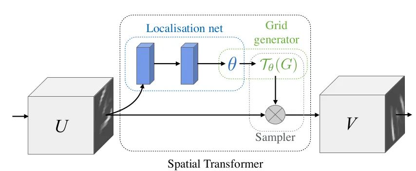
This article proposes the STN module, which explicitly embeds spatial transformations into the network, thereby enhancing the network’s invariance to rotation, translation, scale, etc. It can be understood as an “alignment” operation. The structure of STN is shown in the above image, each STN module consists of a Localisation net, Grid generator, and Sampler. The Localisation net is used to learn the parameters of spatial transformations, which are the six parameters in the above formula. The Grid generator is used for coordinate mapping. The Sampler is used for pixel collection, which is done using bilinear interpolation.

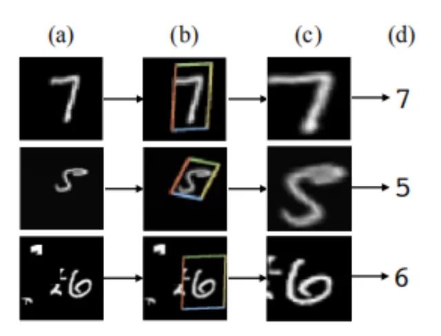
The significance of STN is that it can correct the original image to the ideal image desired by the network, and this process is done in an unsupervised manner, meaning the transformation parameters are learned spontaneously without needing annotated information. This module is an independent module that can be inserted at any position in the CNN. It meets the requirements of this “plugin” summary.

Core Code:

class SpatialTransformer(nn.Module):    def __init__(self, spatial_dims):        super(SpatialTransformer, self).__init__()        self._h, self._w = spatial_dims         self.fc1 = nn.Linear(32*4*4, 1024) # Can set according to your network parameters        self.fc2 = nn.Linear(1024, 6)    def forward(self, x):         batch_images = x # Save a copy of the original data        x = x.view(-1, 32*4*4)        # Use FC structure to learn 6 parameters        x = self.fc1(x)        x = self.fc2(x)         x = x.view(-1, 2,3) # 2x3        # Use affine_grid to generate sampling points        affine_grid_points = F.affine_grid(x, torch.Size((x.size(0), self._in_ch, self._h, self._w)))        # Apply sampling points to the original data        rois = F.grid_sample(batch_images, affine_grid_points)        return rois, affine_grid_points

Full Name of Plugin: atrous spatial pyramid pooling

From Paper: DeepLab: Semantic Image Segmentation with Deep Convolutional Nets, Atrous Conv

Paper Link: https://arxiv.org/pdf/1606.00915.pdf

Core Analysis:

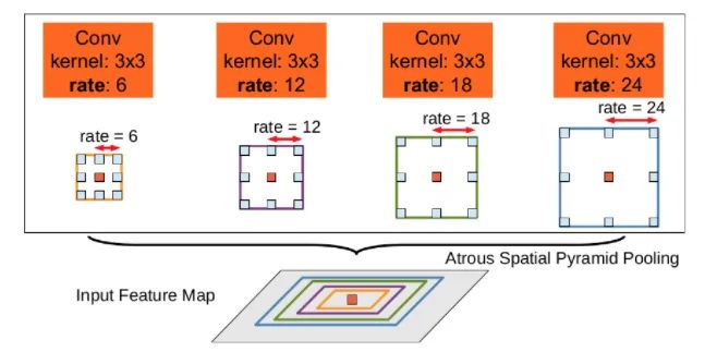
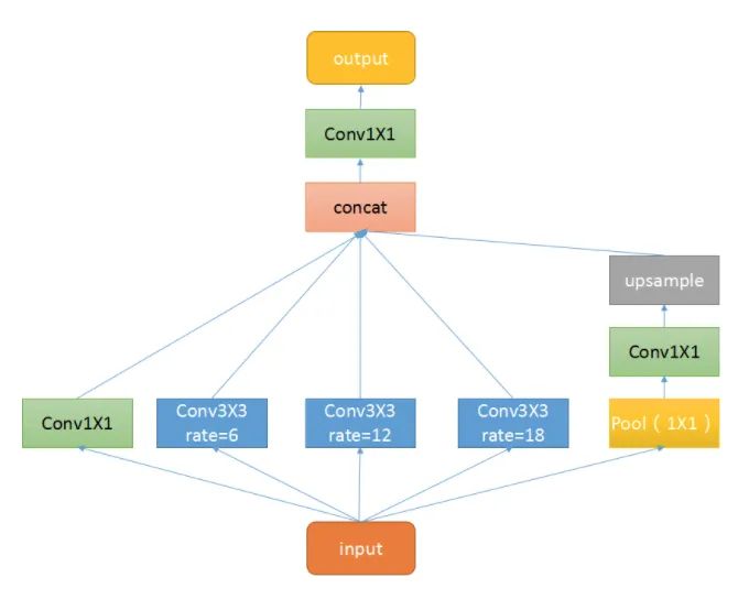
This plugin is a spatial pyramid pooling module with dilated convolution, mainly proposed to enhance the receptive field of the network and introduce multi-scale information. We know that for semantic segmentation networks, they usually face images with high resolution, which requires our networks to have a sufficient receptive field to cover the target objects. CNN networks mainly rely on stacking convolutional layers and downsampling operations to achieve receptive fields. This module can control the receptive field without changing the size of the feature map, which is beneficial for extracting multi-scale information. The rate controls the size of the receptive field; the larger the rate, the larger the receptive field.

ASPP mainly includes the following parts: 1. A global average pooling layer to obtain image-level features, followed by a 1×1 convolution, and bilinearly interpolated to the original size; 2. A 1×1 convolution layer and three 3×3 dilated convolutions; 3. Concatenate the five different scale features along the channel dimension, then send them into a 1×1 convolution for fusion output.

Core Code:

class ASPP(nn.Module):    def __init__(self, in_channel=512, depth=256):        super(ASPP,self).__init__()        self.mean = nn.AdaptiveAvgPool2d((1, 1))        self.conv = nn.Conv2d(in_channel, depth, 1, 1)        self.atrous_block1 = nn.Conv2d(in_channel, depth, 1, 1)        # Convolutions with different dilation rates        self.atrous_block6 = nn.Conv2d(in_channel, depth, 3, 1, padding=6, dilation=6)        self.atrous_block12 = nn.Conv2d(in_channel, depth, 3, 1, padding=12, dilation=12)        self.atrous_block18 = nn.Conv2d(in_channel, depth, 3, 1, padding=18, dilation=18)        self.conv_1x1_output = nn.Conv2d(depth * 5, depth, 1, 1)    def forward(self, x):        size = x.shape[2:]     # Pooling branch        image_features = self.mean(x)        image_features = self.conv(image_features)        image_features = F.upsample(image_features, size=size, mode='bilinear')     # Convolutions with different dilation rates        atrous_block1 = self.atrous_block1(x)        atrous_block6 = self.atrous_block6(x)        atrous_block12 = self.atrous_block12(x)        atrous_block18 = self.atrous_block18(x)        # Combine features of all scales     x = torch.cat([image_features, atrous_block1, atrous_block6,atrous_block12, atrous_block18], dim=1)        # Use 1x1 convolution to fuse feature outputs        x = self.conv_1x1_output(x)        return net

From Paper: Non-local Neural Networks

Paper Link: https://arxiv.org/abs/1711.07971

Core Analysis:

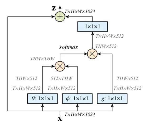
Non-Local is an attention mechanism and also a module that is easy to embed and integrate. Local is mainly aimed at the receptive field. Taking the convolution and pooling operations in CNNs as an example, its receptive field size is the kernel size, while we commonly use 3×3 convolution layers stacked together, which only consider local areas, all local operations. In contrast, non-local operations can have a large receptive field, potentially a global area, rather than a local area. Capturing long-range dependencies, that is, how to establish a connection between two pixels that are a certain distance apart in an image, is an attention mechanism. The so-called attention mechanism generates a saliency map using the network, and attention corresponds to salient areas, which are the regions that the network needs to focus on.

• First, perform a 1×1 convolution on the input feature map to compress the channel number, obtaining features.
• Then, reshape the three features’ dimensions, and perform matrix multiplication to obtain a covariance-like matrix, this step is to calculate the self-correlation in the features, that is, to obtain the relationship of each pixel in each frame to all other pixels in all frames.
• Next, perform a Softmax operation on the self-correlation features to obtain weights between 0 and 1, which are the self-attention coefficients we need.
• Finally, multiply the attention coefficients back to the feature matrix g and add it to the original input feature map X as a residual output.

Here we combine a simple example to understand, assuming g is (we temporarily do not consider batch and channel dimensions):

g = torch.tensor([[1, 2],                           [3, 4]).view(-1, 1).float()

is:

theta = torch.tensor([2, 4, 6, 8]).view(-1, 1)

is:

phi = torch.tensor([7, 5, 3, 1]).view(1, -1)

Then, the matrix multiplication is as follows:

tensor([[14., 10.,  6.,  2.],                [28., 20., 12.,  4.],                [42., 30., 18.,  6.],                [56., 40., 24.,  8.]])

After softmax(dim=-1), it looks as follows, each row represents the importance of elements in g, where the values in front of each row are larger, thus we hope to pay more “attention” to the earlier elements in g, meaning 1 is a bit more important. Alternatively, this can be understood as the attention matrix representing the dependency degree of each element in g to other elements.

tensor([[9.8168e-01, 1.7980e-02, 3.2932e-04, 6.0317e-06],                [9.9966e-01, 3.3535e-04, 1.1250e-07, 3.7739e-11],                [9.9999e-01, 6.1442e-06, 3.7751e-11, 2.3195e-16],                [1.0000e+00, 1.1254e-07, 1.2664e-14, 1.4252e-21]])

After the attention is applied, the overall values converge towards 1 in the original g:

tensor([[1.0187, 1.0003],                [1.0000, 1.0000]])

Core Code:

class NonLocal(nn.Module):    def __init__(self, channel):        super(NonLocalBlock, self).__init__()        self.inter_channel = channel // 2        self.conv_phi = nn.Conv2d(channel, self.inter_channel, 1, 1,0, False)        self.conv_theta = nn.Conv2d(channel, self.inter_channel, 1, 1,0, False)        self.conv_g = nn.Conv2d(channel, self.inter_channel, 1, 1, 0, False)        self.softmax = nn.Softmax(dim=1)        self.conv_mask = nn.Conv2d(self.inter_channel, channel, 1, 1, 0, False)    def forward(self, x):        # [N, C, H , W]        b, c, h, w = x.size()        # Get phi features, dimensions [N, C/2, H * W], note that batch and channel dimensions are retained, it's done on HW        x_phi = self.conv_phi(x).view(b, c, -1)        # Get theta features, dimensions [N, H * W, C/2]        x_theta = self.conv_theta(x).view(b, c, -1).permute(0, 2, 1).contiguous()        # Get g features, dimensions [N, H * W, C/2]        x_g = self.conv_g(x).view(b, c, -1).permute(0, 2, 1).contiguous()        # Perform matrix multiplication of phi and theta, [N, H * W, H * W]        mul_theta_phi = torch.matmul(x_theta, x_phi)        # Softmax to bring it between 0 and 1        mul_theta_phi = self.softmax(mul_theta_phi)        # Perform matrix multiplication with g features, [N, H * W, C/2]        mul_theta_phi_g = torch.matmul(mul_theta_phi, x_g)        # [N, C/2, H, W]        mul_theta_phi_g = mul_theta_phi_g.permute(0, 2, 1).contiguous().view(b, self.inter_channel, h, w)        # 1x1 convolution to expand channel number        mask = self.conv_mask(mul_theta_phi_g)        out = mask + x # Residual connection        return out

From Paper: Squeeze-and-Excitation Networks

Paper Link: https://arxiv.org/pdf/1709.01507.pdf

Core Analysis:

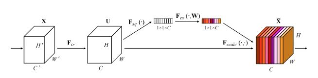
This article is the champion work of the last ImageNet competition, and you will see its presence in many classic network architectures, such as Mobilenet v3. It is actually a type of channel attention mechanism. Due to feature compression and the presence of FC, the captured channel attention features have global information. This article proposes a new structural unit—the “Squeeze-and Excitation (SE)” module, which can adaptively adjust the feature response values of each channel and model the internal dependencies between channels. The steps are as follows:

• Squeeze: Compress features along the spatial dimension, turning each two-dimensional feature channel into a single number, which has a global receptive field.

• Excitation: Each feature channel generates a weight representing the importance of that feature channel.

• Reweight: The weights output from Excitation are treated as the importance of each feature channel and are applied to each channel through multiplication.

Core Code:

class SE_Block(nn.Module):    def __init__(self, ch_in, reduction=16):        super(SE_Block, self).__init__()        self.avg_pool = nn.AdaptiveAvgPool2d(1)  # Global adaptive pooling        self.fc = nn.Sequential(            nn.Linear(ch_in, ch_in // reduction, bias=False),            nn.ReLU(inplace=True),            nn.Linear(ch_in // reduction, ch_in, bias=False),            nn.Sigmoid()        )    def forward(self, x):        b, c, _, _ = x.size()        y = self.avg_pool(x).view(b, c) # squeeze operation        y = self.fc(y).view(b, c, 1, 1) # FC to obtain channel attention weights, which have global information        return x * y.expand_as(x) # Attention applied to each channel

From Paper: CBAM: Convolutional Block Attention Module

Paper Link: https://openaccess.thecvf.com/content_ECCV_2018/papers/Sanghyun_Woo_Convolutional_Block_Attention_ECCV_2018_paper.pdf

Core Analysis:

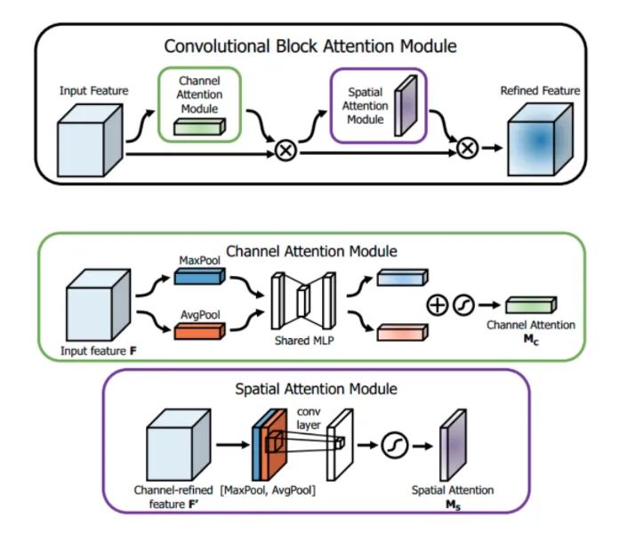
SENet focuses on obtaining attention weights on the channel dimension of the feature map and then multiplying it with the original feature map. This article points out that this attention method only focuses on which layers in the channel dimension have stronger feedback capabilities, but it does not reflect attention in the spatial dimension. CBAM, as the highlight of this article, applies attention simultaneously in both channel and spatial dimensions. Like the SE Module, CBAM can be embedded into most mainstream networks, enhancing the model’s feature extraction capabilities without significantly increasing the computational and parameter load.

Channel Attention: As shown in the above image, the input is a feature F of size H×W×C. We first perform global average pooling and max pooling in two spatial dimensions to obtain two 1×1×C channel descriptions. Then, we send them into a two-layer neural network, where the first layer has C/r neurons and the activation function is Relu, and the second layer has C neurons. Note that this two-layer neural network is shared. Finally, the two obtained features are added together and passed through a Sigmoid activation function to obtain the weight coefficient Mc. Finally, multiply the weight coefficient with the original feature F to get the scaled new feature. Pseudo code:

def forward(self, x):    # Use FC to obtain global information, essentially the same as multiplying with Non-local's matrix    avg_out = self.fc2(self.relu1(self.fc1(self.avg_pool(x))))    max_out = self.fc2(self.relu1(self.fc1(self.max_pool(x))))    out = avg_out + max_out    return self.sigmoid(out)

Spatial Attention: Similar to channel attention, given a feature F’ of size H×W×C, we first perform average pooling and max pooling along the channel dimension to obtain two H×W×1 channel descriptions, and concatenate these two descriptions along the channel dimension. Then, we pass through a 7×7 convolution layer, with the activation function being Sigmoid, to obtain the weight coefficient Ms. Finally, multiply the weight coefficient with the feature F’ to get the scaled new feature. Pseudo code:

def forward(self, x):    # Here we use pooling to obtain global information    avg_out = torch.mean(x, dim=1, keepdim=True)    max_out, _ = torch.max(x, dim=1, keepdim=True)    x = torch.cat([avg_out, max_out], dim=1)    x = self.conv1(x)    return self.sigmoid(x)

Full Name of Plugin: Deformable Convolutional

From Paper:

v1: [Deformable Convolutional Networks]

https://arxiv.org/pdf/1703.06211.pdf

v2: [Deformable ConvNets v2: More Deformable, Better Results]

https://arxiv.org/pdf/1811.11168.pdf

Core Analysis:

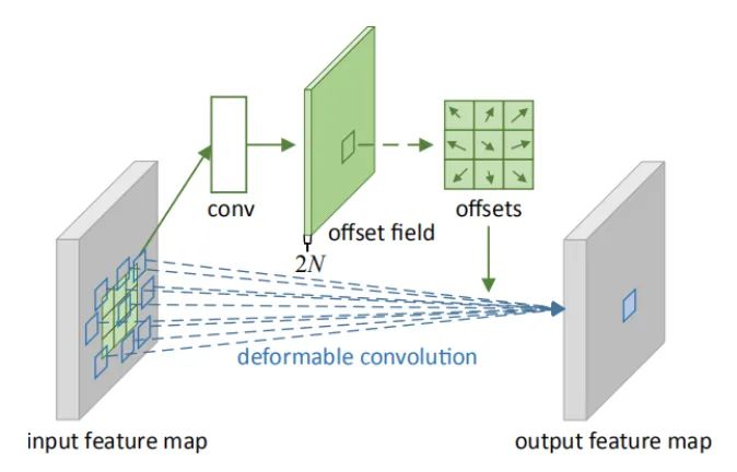
Deformable convolution can be viewed as two parts: deformation + convolution, hence it can be used as a plugin. In major detection networks, deformable convolution is indeed a magic tool for increasing performance, and there are many interpretations online. Compared to traditional fixed-window convolutions, deformable convolutions can effectively adapt to geometric shapes because their “local receptive field” is learnable and aimed at the whole image. This paper also proposes deformable ROI pooling, both methods increase additional offsets for spatial sampling locations, requiring no extra supervision; it is a self-supervised process.

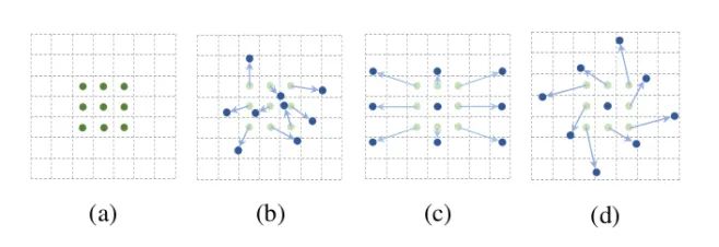
As shown in the above image, a represents different convolutions, b represents deformable convolutions, and the dark points represent the actual sampling positions of the convolution kernel, which are offset from the “standard” positions. c and d represent special forms of deformable convolutions, where c is the commonly seen dilated convolution, and d possesses learning rotation characteristics, also enhancing the receptive field.

Deformable convolution and STN processes are very similar; STN learns six parameters of spatial transformation through the network to perform overall transformations on feature maps, aiming to increase the network’s extraction capability for deformations. DCN learns offsets for the entire image, which is a bit more “comprehensive” than STN. STN is affine transformation, while DCN is arbitrary transformation. I won’t include the formulas; you can directly look at the code implementation process.

Deformable convolution has two versions, V1 and V2, where V2 improves upon V1 by adding sampling weights in addition to sampling offsets. V2 believes that 3×3 sampling points should also have different levels of importance; therefore, this processing method is more flexible and has better fitting capabilities.

Core Code:

def forward(self, x):    # Learn offsets, including x and y directions, note that each pixel in each channel has an x and y offset    offset = self.p_conv(x)    if self.v2: # In V2, an additional weight coefficient is learned, which is sigmoid-transformed to be between 0 and 1        m = torch.sigmoid(self.m_conv(x))    # Use offsets to interpolate x to get the offset x_offset    x_offset = self.interpolate(x, offset)    if self.v2: # In V2, the weight coefficient is applied to the feature map        m = m.contiguous().permute(0, 2, 3, 1)        m = m.unsqueeze(dim=1)        m = torch.cat([m for _ in range(x_offset.size(1))], dim=1)        x_offset *= m    out = self.conv(x_offset) # After applying offsets, proceed with standard convolution process    return out

From Paper: An intriguing failing of convolutional neural networks and the CoordConv solution

Paper Link: https://arxiv.org/pdf/1807.03247.pdf

Core Analysis:

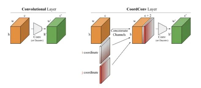
In the Solo semantic segmentation algorithm and Yolov5, you can see its presence. This article starts from several small experiments, exploring the ability of convolutional networks to perform coordinate transformations. It shows that they cannot convert spatial representations into coordinates in Cartesian space. As shown in the image below, we input (i, j) coordinates into a network, requiring it to output a 64×64 image and draw a square or a pixel at the coordinates, but the network fails to accomplish this in the test set. Although this task is something we humans consider extremely simple. The reason is that convolution, as a local and weight-sharing filter applied to the input, does not know where each filter is and cannot capture positional information. Therefore, we can help the convolution to know the position of the filters. We only need to add two channels to the input, one for the i coordinate and one for the j coordinate. The specific approach is shown in the image above, adding two channels before inputting into the filter. This way, the network gains spatial positional information, which is quite magical! You can randomly use this plugin in classification, segmentation, detection, and other tasks.

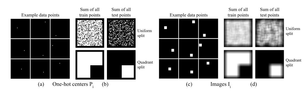
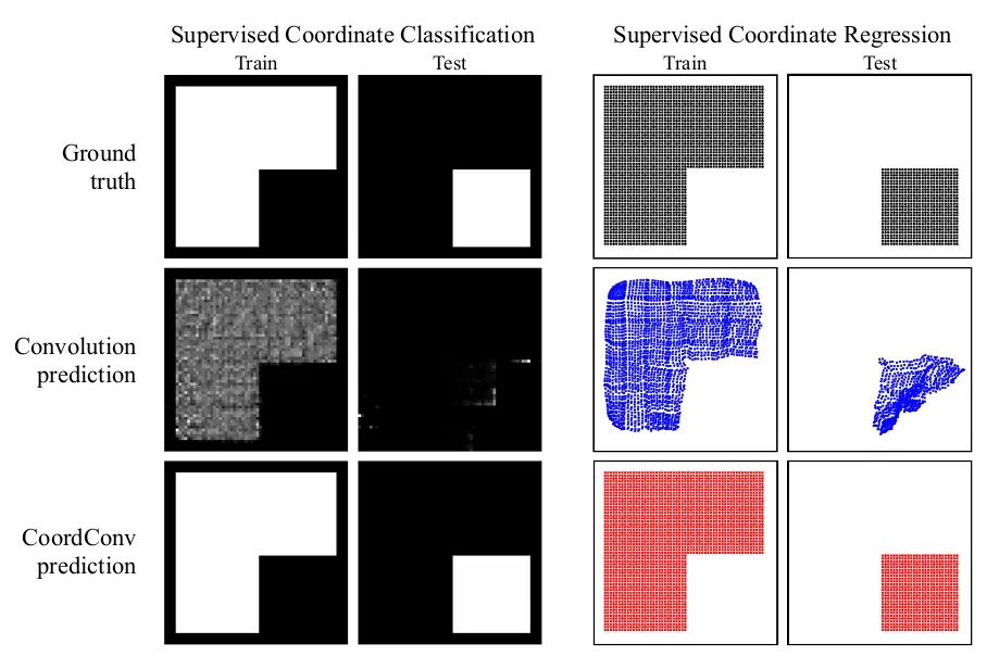
As shown in the first group of images, traditional CNNs struggle to generate images based on coordinate values in the task; they perform well on the training set but poorly on the test set. The second group of images shows that after adding CoordConv, the task can be easily accomplished, demonstrating that it enhances the spatial perception capability of CNNs.

Core Code:

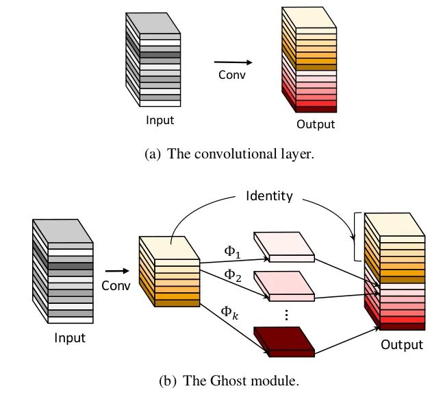
ins_feat = x # Current instance feature tensor# Generate linear values from -1 to 1x_range = torch.linspace(-1, 1, ins_feat.shape[-1], device=ins_feat.device)y_range = torch.linspace(-1, 1, ins_feat.shape[-2], device=ins_feat.device)y, x = torch.meshgrid(y_range, x_range) # Generate a 2D coordinate gridy = y.expand([ins_feat.shape[0], 1, -1, -1]) # Expand to the same dimension as ins_featx = x.expand([ins_feat.shape[0], 1, -1, -1])coord_feat = torch.cat([x, y], 1) # Position featuresins_feat = torch.cat([ins_feat, coord_feat], 1) # Concatenate as input for the next convolution

Full Name of Plugin: Ghost module

From Paper: GhostNet: More Features from Cheap Operations

Paper Link: https://arxiv.org/pdf/1911.11907.pdf

Core Analysis:

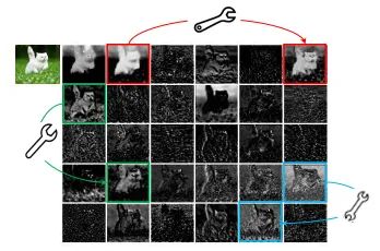
In the ImageNet classification task, GhostNet achieved a Top-1 accuracy of 75.7% with a similar computational load as MobileNetV3’s 75.2%. Its main innovation is the introduction of the Ghost module. In CNN models, feature maps often contain a lot of redundancy, which is indeed very important and necessary. As shown in the image, the feature maps marked with “small wrenches” all have redundant feature maps. So can we reduce the number of convolution channels and then generate redundant feature maps through some transformations? This is essentially the idea of GhostNet.

This article starts from the redundancy issue of feature maps and proposes a structure that can generate a large number of feature maps with only a small amount of computation (referred to as cheap operations in the paper) — the Ghost Module. The cheap operations are linear transformations, implemented in the paper using convolution operations. The specific process is as follows:

• Use fewer convolution operations than the original, for example, normally using 64 convolution kernels, here use 32, reducing the computation by half.

• Use depthwise separable convolutions to transform redundant features from the above.

• Concatenate the features obtained from the above two steps and output them for subsequent processes.

Core Code:

class GhostModule(nn.Module):    def __init__(self, inp, oup, kernel_size=1, ratio=2, dw_size=3, stride=1, relu=True):        super(GhostModule, self).__init__()        self.oup = oup        init_channels = math.ceil(oup / ratio)        new_channels = init_channels*(ratio-1)        self.primary_conv = nn.Sequential(            nn.Conv2d(inp, init_channels, kernel_size, stride, kernel_size//2, bias=False),            nn.BatchNorm2d(init_channels),            nn.ReLU(inplace=True) if relu else nn.Sequential(), )  # Cheap operation, note the use of grouped convolutions for channel separation        self.cheap_operation = nn.Sequential(            nn.Conv2d(init_channels, new_channels, dw_size, 1, dw_size//2, groups=init_channels, bias=False),            nn.BatchNorm2d(new_channels),            nn.ReLU(inplace=True) if relu else nn.Sequential(),)    def forward(self, x):        x1 = self.primary_conv(x)  # Main convolution operation        x2 = self.cheap_operation(x1) # Cheap transformation operation        out = torch.cat([x1,x2], dim=1) # Concatenate both        return out[:,:self.oup,:,:]

From Paper: Making Convolutional Networks Shift-Invariant Again

Paper Link: https://arxiv.org/abs/1904.11486

Core Analysis:

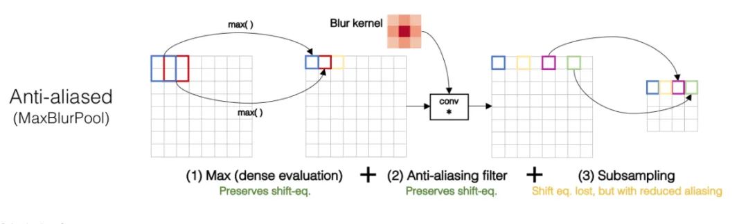
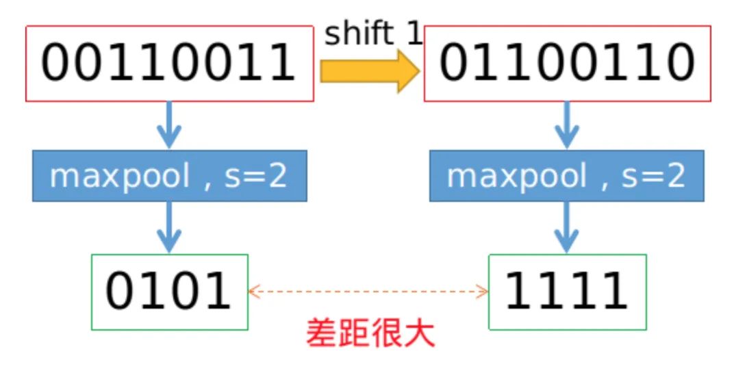
We all know that convolution operations based on sliding windows have translational invariance, thus it is assumed that CNN networks possess translational invariance or equivariance. However, is this really the case? Practice has shown that CNNs are very sensitive; just changing one pixel in the input image or shifting one pixel can lead to significant changes in CNN’s output, even resulting in incorrect predictions. This indicates a lack of robustness. Generally, we use data augmentation to achieve so-called invariance. This article investigates that the degradation of invariance is fundamentally due to downsampling, whether it is Max Pool or Average Pool, or convolutions with a stride > 1; any downsampling involving a stride greater than 1 will lead to the loss of translational invariance. The specific example is shown in the image below; merely shifting one pixel can lead to significant differences in the Max pool results.

To maintain translational invariance, low-pass filtering can be performed before downsampling. Traditional max pooling can be decomposed into two parts: max with stride = 1 + downsampling. Therefore, the authors propose MaxBlurPool = max + blur + downsampling to replace the original max pool. Experiments found that this operation, while not completely solving the loss of translational invariance, can significantly alleviate it.

Core Code:

class BlurPool(nn.Module):    def __init__(self, channels, pad_type='reflect', filt_size=4, stride=2, pad_off=0):        super(BlurPool, self).__init__()        self.filt_size = filt_size        self.pad_off = pad_off        self.pad_sizes = [int(1.*(filt_size-1)/2), int(np.ceil(1.*(filt_size-1)/2)), int(1.*(filt_size-1)/2), int(np.ceil(1.*(filt_size-1)/2))]        self.pad_sizes = [pad_size+pad_off for pad_size in self.pad_sizes]        self.stride = stride        self.off = int((self.stride-1)/2.)        self.channels = channels    # Define a series of Gaussian kernels        if(self.filt_size==1):            a = np.array([1.,])        elif(self.filt_size==2):            a = np.array([1., 1.])        elif(self.filt_size==3):            a = np.array([1., 2., 1.])        elif(self.filt_size==4):            a = np.array([1., 3., 3., 1.])        elif(self.filt_size==5):            a = np.array([1., 4., 6., 4., 1.])        elif(self.filt_size==6):            a = np.array([1., 5., 10., 10., 5., 1.])        elif(self.filt_size==7):            a = np.array([1., 6., 15., 20., 15., 6., 1.])        filt = torch.Tensor(a[:,None]*a[None,:])        filt = filt/torch.sum(filt) # Normalization operation to ensure the information total remains unchanged after blur        # Non-grad operation parameters are stored using buffer        self.register_buffer('filt', filt[None,None,:,:].repeat((self.channels,1,1,1)))        self.pad = get_pad_layer(pad_type)(self.pad_sizes)    def forward(self, inp):        if(self.filt_size==1):            if(self.pad_off==0):                return inp[:,:,::self.stride,::self.stride]                else:                return self.pad(inp)[:,:,::self.stride,::self.stride]        else:            # Use fixed parameter conv2d+stride to implement blurpool            return F.conv2d(self.pad(inp), self.filt, stride=self.stride, groups=inp.shape[1])

Full Name of Plugin: Receptive Field Block

From Paper: Receptive Field Block Net for Accurate and Fast Object Detection

Paper Link: https://arxiv.org/abs/1711.07767

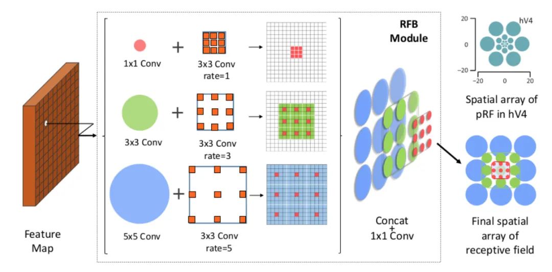
Core Analysis:

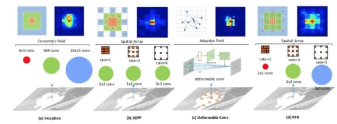
The paper finds that target regions should be as close to the center of the receptive field as possible, which helps enhance the model’s robustness to small-scale spatial displacements. Inspired by the human visual RF structure, this paper proposes the Receptive Field Block (RFB), which strengthens the ability of deep features learned by CNN models, making detection models more accurate. RFB can be used as a universal module embedded in most networks. The image below illustrates its differences from inception, ASPP, and DCN, and can be viewed as a combination of inception and ASPP.

Core Code:

class RFB(nn.Module):    def __init__(self, in_planes, out_planes, stride=1, scale = 0.1, visual = 1):        super(RFB, self).__init__()        self.scale = scale        self.out_channels = out_planes        inter_planes = in_planes // 8        # Branch 0: 1x1 convolution + 3x3 convolution        self.branch0 = nn.Sequential(conv_bn_relu(in_planes, 2*inter_planes, 1, stride),                conv_bn_relu(2*inter_planes, 2*inter_planes, 3, 1, visual, visual, False))        # Branch 1: 1x1 convolution + 3x3 convolution + dilated convolution        self.branch1 = nn.Sequential(conv_bn_relu(in_planes, inter_planes, 1, 1),                conv_bn_relu(inter_planes, 2*inter_planes, (3,3), stride, (1,1)),                conv_bn_relu(2*inter_planes, 2*inter_planes, 3, stride, visual+1,visual+1,False))        # Branch 2: 1x1 convolution + 3x3 convolution*3 instead of 5x5 convolution + dilated convolution        self.branch2 = nn.Sequential(conv_bn_relu(in_planes, inter_planes, 1, 1),                conv_bn_relu(inter_planes, (inter_planes//2)*3, 3, 1, 1),                conv_bn_relu((inter_planes//2)*3, 2*inter_planes, 3, stride, 1),                conv_bn_relu(2*inter_planes, 2*inter_planes, 3, 1, 2*visual+1, 2*visual+1,False))        self.ConvLinear = conv_bn_relu(6*inter_planes, out_planes, 1, 1, False)        self.shortcut = conv_bn_relu(in_planes, out_planes, 1, stride, relu=False)        self.relu = nn.ReLU(inplace=False)    def forward(self,x):        x0 = self.branch0(x)        x1 = self.branch1(x)        x2 = self.branch2(x)    # Scale fusion        out = torch.cat((x0,x1,x2),1)        # 1x1 convolution        out = self.ConvLinear(out)        short = self.shortcut(x)        out = out*self.scale + short        out = self.relu(out)        return out

Full Name of Plugin: Adaptively Spatial Feature Fusion

From Paper: Adaptively Spatial Feature Fusion Learning Spatial Fusion for Single-Shot Object Detection

Paper Link: https://arxiv.org/abs/1911.09516v1

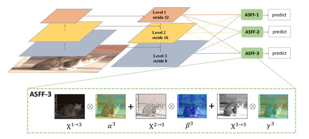
Core Analysis:

To make better use of high-level semantic features and low-level fine-grained features, many networks adopt the FPN approach to output multi-layer features, but they often use concat or element-wise fusion methods. This paper argues that such methods cannot fully utilize features of different scales, thus proposing Adaptively Spatial Feature Fusion, i.e., an adaptive feature fusion method. The feature maps output by FPN undergo the following two processes:

Feature Resizing: Different scales of feature maps cannot be fused element-wise, thus they need to be resized. For upsampling: first, use a 1×1 convolution for channel compression, then use interpolation to upsample the feature map. For 1/2 downsampling: use a 3×3 convolution with stride=2 to simultaneously compress channels and reduce the feature map size. For 1/4 downsampling: insert a max pooling with stride=2 before the 3×3 convolution with stride=2.

Adaptive Fusion: The feature maps are adaptively fused, as per the formula below:

Where x n→l represents the feature vector at position (i, j), coming from the n feature map, resized to scale l. Alpha, Beta, and gamma are spatial attention weights, processed through softmax, as follows:

Code Analysis:

class ASFF(nn.Module):    def __init__(self, level, rfb=False):        super(ASFF, self).__init__()        self.level = level        # Channels of the three input feature layers, modify based on actual conditions        self.dim = [512, 256, 256]        self.inter_dim = self.dim[self.level]        # Output channel numbers of each layer must be consistent        if level==0:            self.stride_level_1 = conv_bn_relu(self.dim[1], self.inter_dim, 3, 2)            self.stride_level_2 = conv_bn_relu(self.dim[2], self.inter_dim, 3, 2)            self.expand = conv_bn_relu(self.inter_dim, 1024, 3, 1)        elif level==1:            self.compress_level_0 = conv_bn_relu(self.dim[0], self.inter_dim, 1, 1)            self.stride_level_2 = conv_bn_relu(self.dim[2], self.inter_dim, 3, 2)            self.expand = conv_bn_relu(self.inter_dim, 512, 3, 1)        elif level==2:            self.compress_level_0 = self.compress_level_0(x_level_0)            self.compress_level_1 = self.compress_level_1(x_level_1)            self.expand = add_conv(self.inter_dim, 256, 3, 1)        compress_c = 8 if rfb else 16          self.weight_level_0 = conv_bn_relu(self.inter_dim, compress_c, 1, 1)        self.weight_level_1 = conv_bn_relu(self.inter_dim, compress_c, 1, 1)        self.weight_level_2 = conv_bn_relu(self.inter_dim, compress_c, 1, 1)        self.weight_levels = nn.Conv2d(compress_c*3, 3, 1, 1, 0)  # Scale sizes level_0 < level_1 < level_2    def forward(self, x_level_0, x_level_1, x_level_2):        # Feature Resizing process        if self.level==0:            level_0_resized = x_level_0            level_1_resized = self.stride_level_1(x_level_1)            level_2_downsampled_inter =F.max_pool2d(x_level_2, 3, stride=2, padding=1)            level_2_resized = self.stride_level_2(level_2_downsampled_inter)        elif self.level==1:            level_0_compressed = self.compress_level_0(x_level_0)            level_0_resized =F.interpolate(level_0_compressed, 2, mode='nearest')            level_1_resized =x_level_1            level_2_resized =self.stride_level_2(x_level_2)        elif self.level==2:            level_0_compressed = self.compress_level_0(x_level_0)            level_0_resized =F.interpolate(level_0_compressed, 4, mode='nearest')            if self.dim[1] != self.dim[2]:                level_1_compressed = self.compress_level_1(x_level_1)                level_1_resized = F.interpolate(level_1_compressed, 2, mode='nearest')            else:                level_1_resized =F.interpolate(x_level_1, 2, mode='nearest')            level_2_resized =x_level_2    # Fusion weights are also learned from the network        level_0_weight_v = self.weight_level_0(level_0_resized)        level_1_weight_v = self.weight_level_1(level_1_resized)        level_2_weight_v = self.weight_level_2(level_2_resized)        levels_weight_v = torch.cat((level_0_weight_v, level_1_weight_v,                                     level_2_weight_v),1)        levels_weight = self.weight_levels(levels_weight_v)        levels_weight = F.softmax(levels_weight, dim=1)   # alpha generated    # Adaptive fusion        fused_out_reduced = level_0_resized * levels_weight[:,0:1,:,:]+\                            level_1_resized * levels_weight[:,1:2,:,:]+\\                            level_2_resized * levels_weight[:,2:,:,:]        out = self.expand(fused_out_reduced)        return out

This article summarizes some of the more exquisite and practical CNN plugins in recent years, hoping everyone can apply them in their actual projects.