
Selected from Medium
Translated by Machine Heart
Contributors: Liu Tianci, Huang Xiaotian
Despite the resurgence and popularity of neural networks in recent years, boosting algorithms still have indispensable advantages in scenarios with limited training sample sizes, shorter training times, and lack of tuning knowledge. This article compares three representative boosting algorithms: CatBoost, LightGBM, and XGBoost, from multiple aspects such as algorithm structure differences, handling of categorical variables by each algorithm, and implementation on datasets; although the conclusions are based on a specific dataset, XGBoost is generally slower than the other two algorithms.
Recently, I participated in the Kaggle competition WIDS Datathon, and by using various boosting algorithms, I finally ranked in the top ten. Since then, I have been very curious about how these algorithms work internally, including parameter tuning and their advantages and disadvantages, which led to this article. Despite the resurgence and popularity of neural networks in recent years, I still pay more attention to boosting algorithms because they have absolute advantages in scenarios with limited training sample sizes, shorter training times, and lack of tuning knowledge.
-
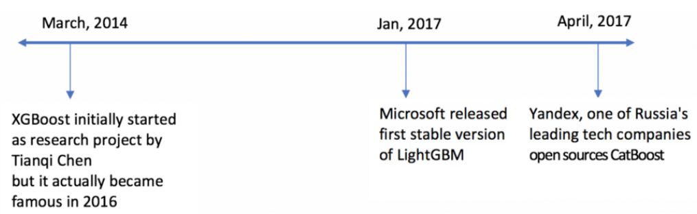
In March 2014, XGBoost was first proposed as a research project by Tianqi Chen.
-
In January 2017, Microsoft released the first stable version of LightGBM.
-
In April 2017, the top Russian tech company Yandex open-sourced CatBoost.
Since XGBoost (commonly known as the GBM killer) has been around in the machine learning field for a long time, there are many detailed articles discussing it, so this article will focus on CatBoost and LGBM. We will discuss:
-
Differences in algorithm structure
-
Handling of categorical variables by each algorithm
-
How to understand parameters
-
Implementation of algorithms on datasets
-
Performance of each algorithm
Structural Differences Between LightGBM and XGBoost
When filtering data samples to find split values, LightGBM uses a novel technique: Gradient-based One-Side Sampling (GOSS); while XGBoost determines the optimal split using pre-sorting algorithms and histogram algorithms. Here, the sample (instance) represents an observation/sample.
First, let’s understand how the pre-sorting algorithm works:
-
For each node, traverse all features
-
For each feature, classify samples based on feature values
-
Perform linear scans to determine the optimal split based on the basic information gain of the current feature
-
Select the best result from all feature split results
In simple terms, the histogram algorithm divides all data points on a certain feature into discrete regions and uses these discrete regions to determine the split values of the histogram. Although the histogram algorithm is more efficient than the pre-sorting algorithm, which requires traversing all possible split points on the pre-sorted feature values, it is still slower than the GOSS algorithm.
Why is the GOSS method so efficient?
In Adaboost, sample weights are a good indicator of sample importance. However, in Gradient Boosted Decision Trees (GBDT), there are no inherent sample weights, so the sampling method used by Adaboost cannot be directly applied here; thus, we need a gradient-based sampling method.
Gradients represent the slope of the loss function’s tangent, so it is natural to infer that if the gradient of a data point is very large in some sense, these samples are very important for determining the optimal split point because their loss is higher.
GOSS retains all samples with large gradients and randomly samples from small gradient samples. For example, if there are 500,000 rows of data, and 10,000 of those have large gradients, my algorithm will select (these 10,000 large gradient rows + x% randomly sampled from the remaining 490,000 rows). If x is set to 10%, then the final selected result is 59,000 rows drawn from 500,000 based on the determined split value.
There is a basic assumption here: If the gradients of training samples in the training set are very small, then the training error of the algorithm on this training set will be very small because training has already been completed.
To maintain the same data distribution, GOSS introduces a constant factor on small gradient data samples when calculating information gain. Therefore, GOSS achieves a good balance between reducing the number of data samples and maintaining the accuracy of the learned decision tree.
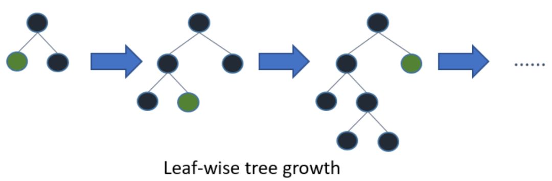
High gradient/error leaves for further growth in LGBM
How does each model handle categorical variable attributes?
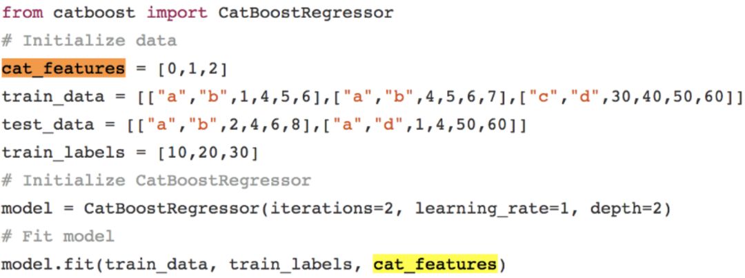
CatBoost
CatBoost can assign indicators to categorical variables, thus obtaining one-hot encoded results through one-hot maximum (one-hot maximum: using one-hot encoding for different numbers less than or equal to a given parameter value across all features).
If the “skip” option is not set in the CatBoost statement, CatBoost will treat all columns as numerical variables.
Note that if a column contains string values, the CatBoost algorithm will throw an error. Additionally, int type variables with default values will also be treated as numerical data by default. In CatBoost, variables must be declared for the algorithm to treat them as categorical variables.
For categorical variables with more unique values than one-hot maximum, CatBoost uses a very effective encoding method similar to mean encoding but can reduce overfitting. The specific implementation is as follows:
1. Randomly shuffle the input sample set and generate multiple groups of random arrangements.
2. Convert floating-point or attribute values into integers.
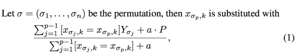
3. Convert all categorical feature value results into numerical results according to the following formula.
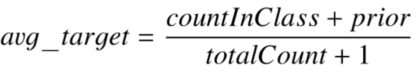
Where CountInClass indicates how many samples in the current categorical feature value have a label value of “1”; Prior is the initial value of the numerator, determined by initial parameters. TotalCount is the number of samples with the same categorical feature value as the current sample among all samples (including the current sample).
This can be expressed with the following mathematical formula:
LightGBM
Similar to CatBoost, LightGBM can also handle attribute data using feature names as input; it does not perform one-hot encoding, so it is much faster than one-hot encoding. LGBM uses a special algorithm to determine the split values of attribute features.
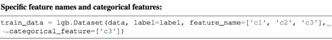
Note that before building a dataset suitable for LGBM, categorical variables need to be converted to integer variables; this algorithm does not allow string data to be passed to categorical variable parameters.
XGBoost
Unlike CatBoost and LGBM algorithms, XGBoost itself cannot handle categorical variables and only accepts numerical data like random forests. Therefore, categorical data must be processed through various encoding methods before being passed to XGBoost: for example, label encoding, mean encoding, or one-hot encoding.
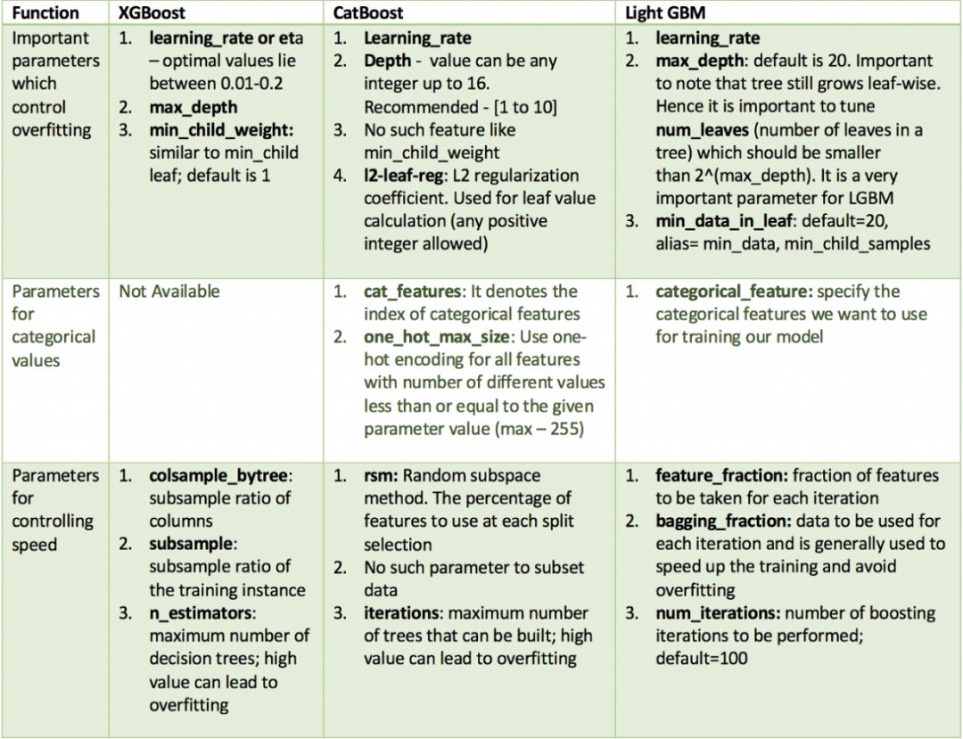
Similarities in Hyperparameters
All of these models require tuning a large number of parameters, but we will only discuss the important ones. Below is a table organizing the important parameters of different algorithms by function.
Implementation
Here, I used the Kaggle dataset on flight delays from 2015, which contains both categorical and numerical variables. This dataset has about 5 million records, making it suitable for simultaneously evaluating and comparing the training speed and accuracy of the three boosting algorithms. I used 10% of the data: 500,000 rows of records.
Below are the features used for modeling:
-
Month, Day, Weekday: integer data
-
Airline or Flight Number: integer data
-
Departure, Arrival Airport: numerical data
-
Departure Time: floating-point data
-
Arrival Delay: this feature is used as the prediction target and converted to a binary variable: whether the flight is delayed by more than 10 minutes
-
Distance and Flight Time: floating-point data
import pandas as pd, numpy as np, time
from sklearn.model_selection import train_test_split

data = pd.read_csv("flights.csv")
data = data.sample(frac = 0.1, random_state=10)

data = data[["MONTH","DAY","DAY_OF_WEEK","AIRLINE","FLIGHT_NUMBER","DESTINATION_AIRPORT",
                 "ORIGIN_AIRPORT","AIR_TIME", "DEPARTURE_TIME","DISTANCE","ARRIVAL_DELAY"]]
data.dropna(inplace=True)

data["ARRIVAL_DELAY"] = (data["ARRIVAL_DELAY"]>10)*1

cols = ["AIRLINE","FLIGHT_NUMBER","DESTINATION_AIRPORT","ORIGIN_AIRPORT"]
for item in cols:
    data[item] = data[item].astype("category").cat.codes +1

train, test, y_train, y_test = train_test_split(data.drop(["ARRIVAL_DELAY"], axis=1), data["ARRIVAL_DELAY"],
                                                random_state=10, test_size=0.25)
XGBoost
import xgboost as xgb
from sklearn import metrics

def auc(m, train, test):
    return (metrics.roc_auc_score(y_train,m.predict_proba(train)[:,1]),
                            metrics.roc_auc_score(y_test,m.predict_proba(test)[:,1]))

# Parameter Tuning
model = xgb.XGBClassifier()
param_dist = {"max_depth": [10,30,50],
              "min_child_weight" : [1,3,6],
              "n_estimators": [200],
              "learning_rate": [0.05, 0.1,0.16],}
grid_search = GridSearchCV(model, param_grid=param_dist, cv = 3,
                                   verbose=10, n_jobs=-1)
grid_search.fit(train, y_train)

grid_search.best_estimator_

model = xgb.XGBClassifier(max_depth=50, min_child_weight=1,  n_estimators=200,
                          n_jobs=-1 , verbose=1,learning_rate=0.16)
model.fit(train,y_train)

auc(model, train, test)
Light GBM
import lightgbm as lgb
from sklearn import metrics

def auc2(m, train, test):
    return (metrics.roc_auc_score(y_train,m.predict(train)),
                            metrics.roc_auc_score(y_test,m.predict(test)))

lg = lgb.LGBMClassifier(silent=False)
param_dist = {"max_depth": [25,50, 75],
              "learning_rate" : [0.01,0.05,0.1],
              "num_leaves": [300,900,1200],
              "n_estimators": [200]
             }
grid_search = GridSearchCV(lg, n_jobs=-1, param_grid=param_dist, cv = 3, scoring="roc_auc", verbose=5)
grid_search.fit(train,y_train)
grid_search.best_estimator_

d_train = lgb.Dataset(train, label=y_train)
params = {"max_depth": 50, "learning_rate" : 0.1, "num_leaves": 900,  "n_estimators": 300}

# Without Categorical Features
model2 = lgb.train(params, d_train)
auc2(model2, train, test)

#With Categorical Features
cate_features_name = ["MONTH","DAY","DAY_OF_WEEK","AIRLINE","DESTINATION_AIRPORT",
                 "ORIGIN_AIRPORT"]
model2 = lgb.train(params, d_train, categorical_feature = cate_features_name)
auc2(model2, train, test)
CatBoost
When tuning parameters for CatBoost, it is difficult to assign indicators to categorical features. Therefore, I provided tuning results without passing categorical features and evaluated two models: one with categorical features and one without. I separately adjusted one-hot maximum as it does not affect other parameters.
import catboost as cb
cat_features_index = [0,1,2,3,4,5,6]

def auc(m, train, test):
    return (metrics.roc_auc_score(y_train,m.predict_proba(train)[:,1]),
                            metrics.roc_auc_score(y_test,m.predict_proba(test)[:,1]))

params = {'depth': [4, 7, 10],
          'learning_rate' : [0.03, 0.1, 0.15],
         'l2_leaf_reg': [1,4,9],
         'iterations': [300]}
cb = cb.CatBoostClassifier()
cb_model = GridSearchCV(cb, params, scoring="roc_auc", cv = 3)
cb_model.fit(train, y_train)

With Categorical features
clf = cb.CatBoostClassifier(eval_metric="AUC", depth=10, iterations= 500, l2_leaf_reg= 9, learning_rate= 0.15)
clf.fit(train,y_train)
auc(clf, train, test)

With Categorical features
clf = cb.CatBoostClassifier(eval_metric="AUC",one_hot_max_size=31, \
                            depth=10, iterations= 500, l2_leaf_reg= 9, learning_rate= 0.15)
clf.fit(train,y_train, cat_features= cat_features_index)
auc(clf, train, test)
Conclusion
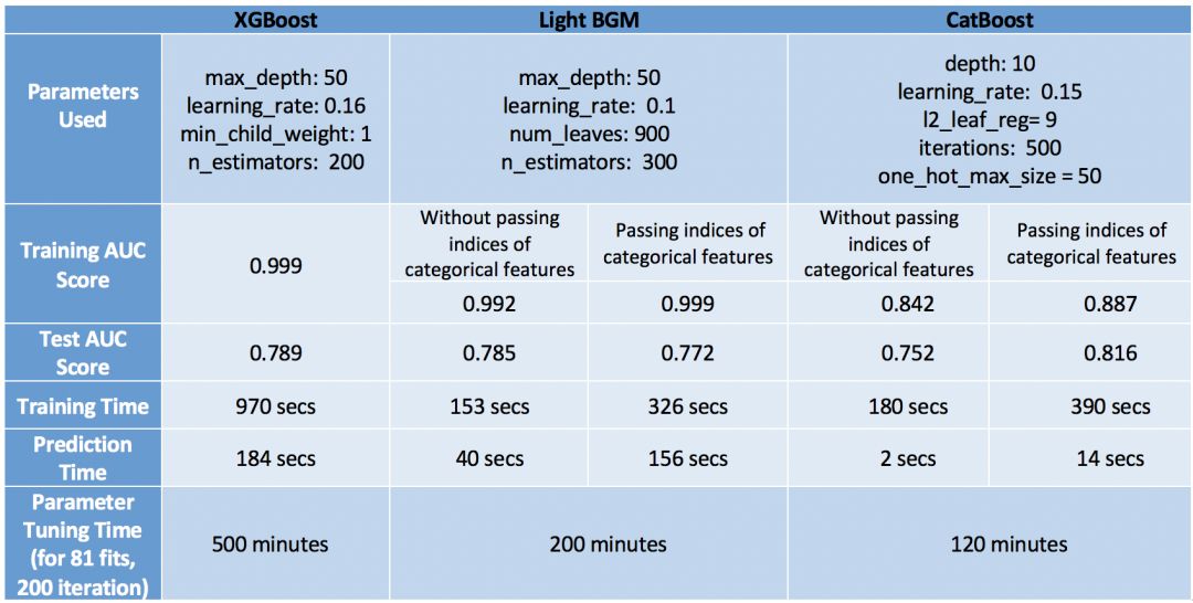
To evaluate models, we should consider both the speed and accuracy performance of the models.
Remember that CatBoost performed the best on the test set, achieving the highest accuracy (0.816), minimal overfitting (accuracy on training and test sets is very close), and minimal prediction and debugging time. However, this performance only occurs when there are categorical features and the one-hot maximum is tuned. If the advantages of the CatBoost algorithm on these features are not utilized, its performance will become the worst: with only 0.752 accuracy. Therefore, we believe that CatBoost will only perform well when the data contains categorical variables, and we have appropriately tuned these variables.
The second model is XGBoost, which also performed quite well. Even without considering that the dataset contains categorical variables that can be used after being converted to numerical variables, its accuracy is very close to that of CatBoost. However, the only problem with XGBoost is that it is too slow. Especially tuning it is very frustrating (I spent 6 hours running GridSearchCV—too terrible). A better choice is to tune parameters separately rather than using GridSearchCV.
The last model is LightGBM. One thing to note here is that when using CatBoost features, LightGBM performed poorly in both training speed and accuracy. I believe this is because it uses some modified mean encoding methods in categorical data, leading to overfitting (the accuracy on the training set is very high: 0.999, especially compared to the accuracy on the test set). However, if we use LightGBM normally, as we do with XGBoost, it will achieve similar accuracy faster than XGBoost, if not higher (LGBM—0.785, XGBoost—0.789).
Finally, it must be pointed out that these conclusions hold for this specific dataset; they may or may not be correct for other datasets. However, in most cases, XGBoost is generally slower than the other two algorithms.
So, which algorithm do you prefer?
Original article address: https://towardsdatascience.com/catboost-vs-light-gbm-vs-xgboost-5f93620723db
This article is translated by Machine Heart, please contact this public account for authorization.
✄————————————————
Join Machine Heart (Full-time reporter/intern): [email protected]
Submissions or inquiries: [email protected]
Advertising & Business Cooperation: [email protected]