Click the above “Little White Learns Vision“, choose to add “Starred” or “Top“
Heavyweight content delivered first-hand
The optimization of machine learning (objective) can be simply described as: searching for a set of parameters w for the model that can significantly reduce the cost function J(w). This cost function usually includes performance evaluation over the entire training set (empirical risk) and additional regularization (structural risk). Unlike traditional optimization, it does not simply solve for the optimal solution based on data; in most machine learning problems, we focus on optimizing performance measure P on the test set (unknown data).
-
For the model, the test set is unknown, and we can only optimize the performance measure P_train on the training set. Under the assumption of independent and identically distributed data, we expect the test set to also perform well (generalization effect), which means we do not blindly pursue the optimal solution for the training set. -
Additionally, in some cases, the performance measure P (such as classification error f1-score) cannot be efficiently optimized. In such cases, we typically optimize a surrogate loss function. For example, negative log-likelihood is often used as a substitute for 0-1 classification loss.
When our learning objective in machine learning is to maximize the reduction of (empirical) loss function, this is similar to traditional optimization. So how do we achieve this goal? Our first reaction might be to directly solve the formula/analytical solution for the minimum of the loss function (like least squares) to obtain the optimal model parameters. However, the loss functions of machine learning models are usually complex, making it difficult to directly find the optimal solution. Fortunately, we can also optimize model parameters through optimization algorithms (such as genetic algorithms, gradient descent algorithms, Newton’s method, etc.) with a limited number of iterations to reduce the value of the loss function as much as possible, obtaining relatively optimal parameter values (numerical solution). The algorithms used to search for a set of optimal parameter solutions w are optimization algorithms. Below is a summary of optimization algorithms: (The figure is consistent with the content of this article, excerpted from @teekee)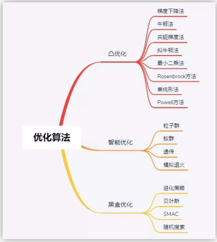
II. Overview of Optimization Algorithms
Least Squares Method
The least squares method is commonly used to find analytical solutions for regression models in machine learning (it cannot be solved by this method for complex deep neural networks). Its geometric significance is the projection of a vector in high-dimensional space onto a low-dimensional subspace.
As an example, let’s solve a univariate linear regression using the least squares method.
The loss function mse is: To minimize the loss function, we set the first derivative to 0. By taking the partial derivative, we can obtain a system of equations about parameters a and bias b:
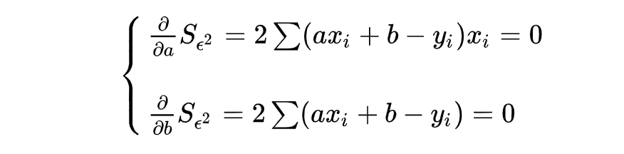 Substituting values into the linear equation system allows us to solve for the parameter values a and b, which correspond to the fitted line ax + b shown in the figure above.
Genetic Algorithms
Note: Gradient descent-based algorithms are relatively efficient for neural network optimization and are mainstream methods. Genetic algorithms, greedy algorithms, simulated annealing, and other optimization methods are used less frequently.
Genetic algorithms (GA) are a type of parallel random search optimization method that simulates the principles of heredity and biological evolution in nature. Similar to the biological evolution principle of “survival of the fittest,” genetic algorithms introduce optimization parameters to form a coding string population, which is filtered according to the selected fitness function through selection, crossover, and mutation in heredity. Individuals with good fitness are retained, while those with poor fitness are eliminated. The new population inherits information from the previous generation while also improving upon it. This process continues iteratively until certain conditions are met.
Gradient Descent (GD)
The gradient descent algorithm can be intuitively understood as a method of going downhill, where the loss function J(w) is likened to a mountain, and our goal is to reach the foot of this mountain (i.e., to solve for the optimal model parameters w that minimize the loss function).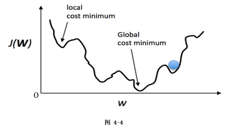
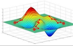
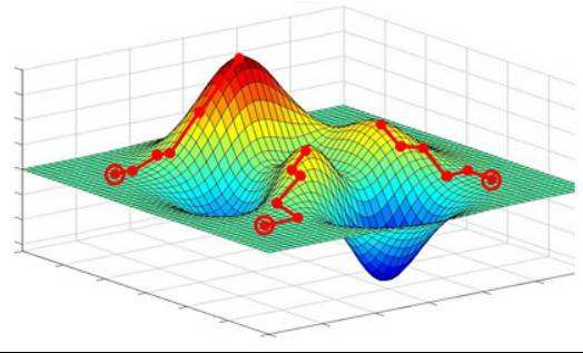
Going downhill simply involves “walking down the slope, taking one step at a time.” On the mountain represented by the loss function, the downhill direction at each position is its negative gradient direction (in simpler terms, the direction that slopes downwards). At each step down, we calculate the gradient at the current position and take a step further in the steepest direction downwards. This process continues until we feel we have reached the foot of the mountain. However, it is possible that we do not reach the foot of the mountain (global optimum, Global cost minimum) but rather arrive at a small valley (local optimum, Local cost minimum), which is a point for further tuning of the gradient descent algorithm. The corresponding algorithm steps are illustrated in my previous figure: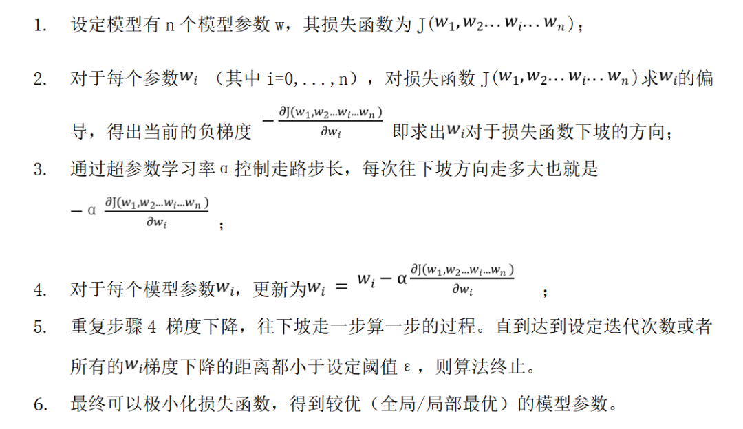 Gradient descent is a broad category, with common gradient descent algorithms and their advantages and disadvantages illustrated in the following figure:
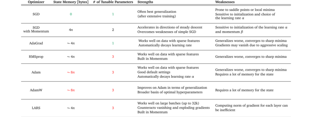
Stochastic Gradient Descent (SGD)
For deep learning, “Stochastic Gradient Descent, SGD” is essentially stochastic gradient descent based on mini-batches (mini-batch SGD), where the batch size is 1, which corresponds to online learning optimization.
Stochastic gradient descent optimizes the efficiency of the gradient descent algorithm by not using the entire sample to compute the current gradient but instead using a mini-batch of samples to estimate the gradient, greatly improving efficiency. The reason is that the returns from estimating the gradient using more samples are less than linear. For most optimization algorithms based on gradient descent, if the time taken to calculate the gradient in each step is significantly reduced, they will converge faster. Additionally, the training set often contains redundancy, with many samples contributing very similarly to the gradient. In this case, the strategy of estimating the gradient based on mini-batch samples can still compute the correct gradient while saving a lot of time.
The choice of batch size for mini-batch is to find the best balance between memory efficiency (time) and memory capacity (space).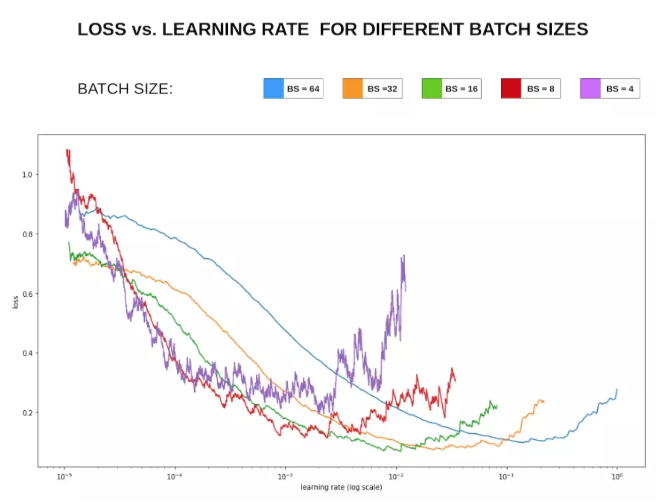
-
Batch size cannot be too large. A larger batch may speed up training but may lead to a decrease in generalization ability. A larger batch size only requires fewer iterations to converge the training error and can leverage the advantages of large-scale data parallelism. However, a larger batch size results in a more accurate gradient estimate, which brings smaller gradient noise. In this case, the noise is too small to push the parameters out of a sharp local minimum’s attraction zone. This situation requires an increase in the learning rate and a decrease in batch size to enhance the contribution of gradient noise.
-
Batch size cannot be too small. A smaller batch size can provide gradient noise similar to a regularization effect, leading to better generalization ability. However, for multi-core architectures, a very small batch does not correspondingly reduce computation time (considering the synchronization overhead between cores). Additionally, a very small batch size results in a high variance in gradient estimates, necessitating a very small learning rate to maintain stability. If the learning rate is too large, it can lead to drastic changes in step size.
Batch size can also be adaptively adjusted; refer to “Small Batch or Large Batch? Peifeng Yin”
Momentum Algorithm
The Momentum algorithm introduces the concept of momentum from physics into gradient descent, simulating the inertia of an object in motion. This means that during updates, a certain degree of the previous update direction is retained while adjusting the previous gradient using the current batch’s gradient. This can increase stability to some extent, allowing for faster learning and providing some ability to escape local optima.
This algorithm introduces a variable v as the velocity vector that continuously moves in the parameter space. The velocity is generally set as the exponential decay moving average of the negative gradient. For a given cost function that needs to be minimized, momentum can be expressed as: updated gradient = decay coefficient γ momentum term + learning rate ŋ current gradient.
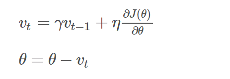
Where ŋ is the learning rate, γ ∈ (0, 1] is the momentum coefficient, and v is the velocity vector. Generally, the direction of descent in the gradient descent algorithm is the direction of steepest descent (mathematically called the steepest descent method). The descent direction at each descent point is perpendicular to the corresponding contour line, which leads to the sawtooth phenomenon of the GD algorithm. Adding momentum to gradient descent is one of the strategies to direct the gradient towards the optimal solution.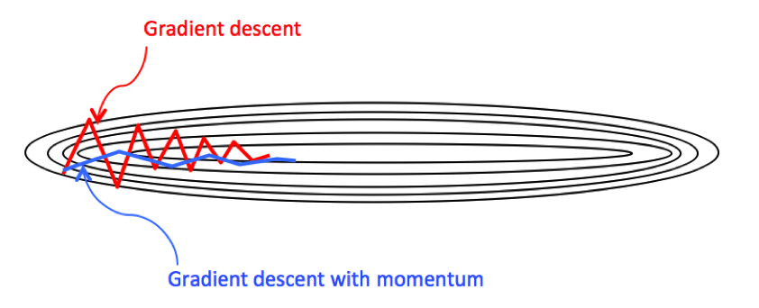
Nesterov
Nesterov momentum is a variant of the momentum method, also known as Nesterov Accelerated Gradient (NAG). Before predicting the next position of the parameter, we already have the current parameter and momentum term. We first use (θ−γvt−1) to predict the next position, which, although not accurate, is generally in the right direction. Then, we use the predicted value at the next moment to calculate the partial derivative, allowing the optimizer to progress efficiently and converge.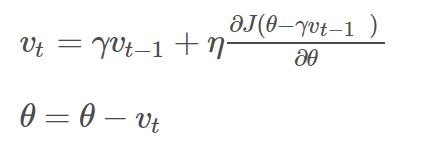
In the optimization of smooth convex functions, compared to batch gradient descent, NAG’s convergence speed exceeds 1/k to 1/(k^2).
Adagrad
Adagrad, also known as adaptive gradient, allows the learning rate to adjust based on parameters without needing to manually adjust the learning rate during the learning process. Adagrad updates the learning rate significantly for infrequently used parameters and slightly for frequently used parameters. However, the main issue with Adagrad is that, in some cases, the learning rate becomes too small, and the monotonically decreasing learning rate causes the network to stop learning.
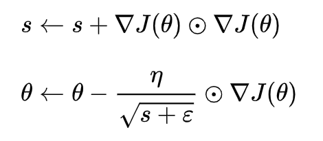
Here, s is the accumulation of squared gradients, and during parameter updates, the learning rate is divided by the square root of this accumulation, with a small value ε added to prevent division by zero. Since s gradually increases, the learning rate decays relatively quickly.
RMSProp
RMSProp is considered an improvement over the Adagrad algorithm, primarily addressing the issue of rapid decay of the learning rate. Instead of directly accumulating squared gradients like the Adagrad algorithm, it adds a decay coefficient γ to control how much historical information is retained.
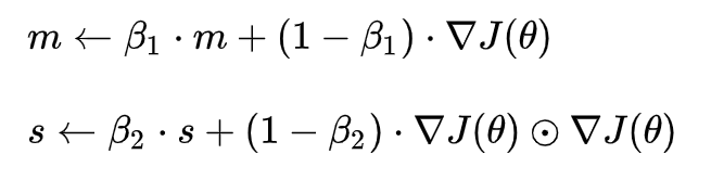
Adam
The Adam algorithm combines the advantages of two types of stochastic gradient descent:
-
The adaptive gradient algorithm (AdaGrad) retains a learning rate for each parameter to enhance performance on sparse gradients (such as in natural language and computer vision problems). -
Root Mean Square Propagation (RMSProp) adaptively retains a learning rate based on the recent magnitude of the weight gradients for each parameter. This means the algorithm performs excellently on non-stationary and online problems.
The Adam algorithm simultaneously gains the advantages of both the AdaGrad and RMSProp algorithms, storing the exponential decay average of past gradients’ squares v, and also retaining the exponential decay average m of past gradients like momentum:
If m and v are initialized as zero vectors, they will be biased towards zero, so bias correction is performed to amplify them: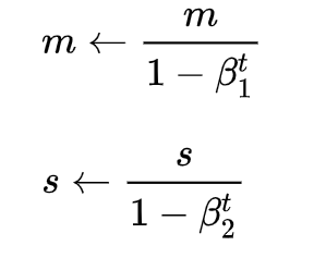
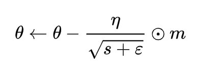
Gradient updates can be adaptively adjusted from both the gradient mean and the squared gradient, rather than being directly determined by the current gradient.
Newton’s Method
Newton’s method, compared to gradient descent, both are iterative solving methods, but gradient descent is a first-order optimization using gradients, while Newton’s method uses the inverse of the Hessian matrix (second-order). Relatively speaking, Newton’s method converges faster (with fewer iterations), but each iteration takes longer than gradient descent (greater computational overhead; the quasi-Newton method is often used instead).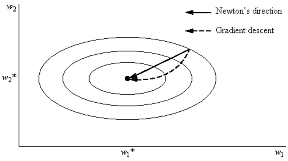
In simpler terms, gradient descent chooses the steepest direction from your current position to step forward, while Newton’s method considers not only the steepness but also whether the slope will become steeper after taking a step. Therefore, it can be said that Newton’s method looks further ahead and can reach the bottom faster. However, Newton’s method has certain requirements for initial values and can easily get stuck in saddle points in non-convex optimization problems (like training neural networks), while gradient descent is more likely to escape saddle points (hence gradient descent is generally used in training neural networks, as there are many saddle points in high-dimensional spaces).
In summary, for the optimization of neural networks, commonly used methods include efficient ones like gradient descent. Gradient descent algorithm categories include SGD, Momentum, Adam, and others. For most tasks, it is generally advisable to try Adam first, then verify the effects of different optimizers on specific tasks.
Download 1: OpenCV-Contrib Extension Module Chinese Version Tutorial

Reply "Extension Module Chinese Tutorial" in the "Little White Learns Vision" public account backend to download the first Chinese version of the OpenCV extension module tutorial online, covering installation of extension modules, SFM algorithms, stereo vision, object tracking, biological vision, super-resolution processing, and more than twenty chapters of content.

Download 2: Python Vision Practical Project 52 Lectures

Reply "Python Vision Practical Project" in the "Little White Learns Vision" public account backend to download 31 visual practical projects including image segmentation, mask detection, lane line detection, vehicle counting, eyeliner addition, license plate recognition, character recognition, emotion detection, text content extraction, face recognition, etc., to help quickly learn computer vision.

Download 3: OpenCV Practical Project 20 Lectures

Reply "OpenCV Practical Project 20 Lectures" in the "Little White Learns Vision" public account backend to download 20 practical projects based on OpenCV to advance OpenCV learning.

Group Chat

Welcome to join the public account reader group to communicate with peers. Currently, there are WeChat groups for SLAM, 3D vision, sensors, autonomous driving, computational photography, detection, segmentation, recognition, medical imaging, GAN, algorithm competitions, etc. (these will gradually be subdivided). Please scan the WeChat ID below to join the group, and note: "nickname + school/company + research direction," for example: "Zhang San + Shanghai Jiao Tong University + Visual SLAM." Please follow the format for notes; otherwise, you will not be approved. After successful addition, you will be invited into relevant WeChat groups based on your research direction. Please do not send advertisements in the group; otherwise, you will be removed. Thank you for your understanding~