

In recent years, with the resurgence of the concept of “Artificial Intelligence”, besides the popular term “Deep Learning”, “Knowledge Graph” has undoubtedly become another “silver bullet” in the minds of researchers, industry professionals, and investors. Simply put, a “Knowledge Graph” is a way to represent “entities”, their “attributes”, and the “relationships” between entities in a graphical format (Graph). The following image is an example taken from Google’s Knowledge Graph introduction webpage. In the example, there are four entities: “Da Vinci”, “Italy”, “Mona Lisa”, and “Michelangelo”. This graph clearly displays the attributes and attribute values of “Da Vinci” (such as name, birth date, and death date), as well as the relationships between them (for example, Mona Lisa is a painting by Da Vinci, and Da Vinci was born in Italy). When I talk about this, I believe many readers will unconsciously relate it to the concept of “ER Diagram” (Entity-Relationship Diagram) in database courses. From a certain perspective, the two indeed have similarities. According to traditional database theory, when we map real-world objects to the information world, the two most important aspects to focus on are: entities (including entity attributes) and entity relationships; and the ER diagram is the most classic conceptual model reflecting entities and entity relationships. We call the ER diagram a conceptual model because its design is meant for humans to understand the objective world, not for computer implementation. Throughout the history of database management systems, hierarchical models, network models, and relational models have emerged; these are computer models implemented by database management systems (DBMS). Therefore, in actual database application projects, there exists a conversion problem from conceptual models to implementation models, such as how to construct relational tables based on ER diagrams. From this perspective, Knowledge Graphs differ from ER diagrams because Knowledge Graphs not only explicitly depict entities and entity relationships, but also define a data model that can be implemented by computers (i.e., the RDF triple data model proposed by W3C), which is the content introduced in Chapter 1 of this article. Since the author’s research background is in databases, this article attempts to introduce the relevant concepts of Knowledge Graphs and the issues in research and application from the perspective of data management. At the same time, because Knowledge Graphs themselves are an interdisciplinary research topic, this article will also introduce the focus of different disciplines (including natural language processing, knowledge engineering, and machine learning) in Knowledge Graph research.
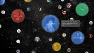
Figure: Example of Google’s Knowledge Graph
This article first introduces the data model of Knowledge Graphs in Chapter 1; Chapter 2 focuses on several case studies of Knowledge Graphs in the industry; Chapter 3 discusses the data management issues facing massive Knowledge Graphs; Chapter 4 provides an overview of the focus of different disciplines in Knowledge Graph research; Chapter 5 concludes the article.

1
Data Model of Knowledge Graphs
The term “Knowledge Graph” became popular due to the launch of Google’s “Knowledge Graph” project on May 16, 2012. Currently, Knowledge Graphs commonly use the RDF (Resource Description Framework) model within the semantic web framework to represent data. The semantic web is a concept proposed by Tim Berners-Lee, the father of the World Wide Web, in 1998, with the core idea of constructing a data-centric web, known as the Web of Data; this is proposed in contrast to our current World Wide Web, which is the Web of Pages. As is well known, the World Wide Web links different documents together using hyperlink technology, making it convenient for users to browse and share documents. The syntax of HTML documents is to inform the browser how to format the document for display, rather than to inform the computer what semantic information the data in the document represents. The core of the semantic web is to enable computers to understand the data in documents and the semantic relationships between data, allowing machines to process this information more intelligently. Therefore, we can imagine the semantic web as a global database system, which is what we usually refer to as the Web of Data. Since semantic web technology involves a wide range of areas, this article will only cover one core concept in the semantic web framework adopted by Knowledge Graphs: RDF (Resource Description Framework). The basic data model of RDF includes three types of objects: Resource, Predicate, and Statements.
Resource: All objects that can be represented using RDF are called resources, including all information on the web, virtual concepts, real-world objects, etc. Resources are represented by unique URIs (Uniform Resource Identifiers, of which the commonly used URLs are a subset), and different resources have different URIs.
Predicate: Predicates describe the characteristics of resources or the relationships between resources. Each predicate has its meaning, used to define the property values of the resource on the predicate or the relationships with other resources.
Statement: A statement consists of three parts, commonly referred to as an RDF triple
The following Figure 1 shows an RDF triple knowledge graph dataset for a person. For example, y:Abraham_Lincoln represents an entity URI (where y indicates the prefix http://en.wikipedia.org/wiki/), which has three attributes (hasName, BornOnDate, DiedOnDate) and one relationship (DiedIn).
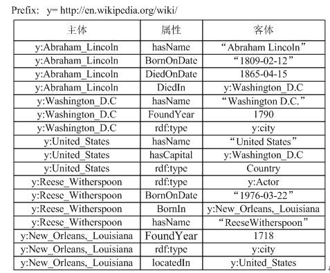
Figure 1: Example of RDF data
For RDF datasets, W3C proposed a structured query language called SPARQL; it is similar to SQL, the query language for relational databases. Like SQL, SPARQL is also a descriptive structured query language, meaning that users only need to describe the information they want to query according to the syntax rules defined by SPARQL, without needing to explicitly specify the implementation steps of the query by the computer. In January 2008, SPARQL became an official W3C standard. The WHERE clause in SPARQL defines the query conditions, which are also represented by triples. We will not delve into the syntax details; interested readers can refer to [1]. The following example illustrates the SPARQL language. Suppose we want to query “the names of people born on February 12, 1809, and who died on April 15, 1865” in the above RDF data. This query can be expressed as the SPARQL statement shown in Figure 2.
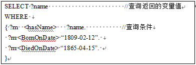
Figure 2: Example of SPARQL query
We can also represent RDF and SPARQL in graphical form. For example, in RDF, subjects and objects can be represented as nodes in the RDF graph, and a statement (i.e., RDF triple) can be represented as an edge, with the predicate as the label of the edge. SPARQL statements can also be represented as a query graph. Figure 3 shows the RDF graph and SPARQL query graph structure corresponding to the above example. Answering SPARQL queries essentially involves finding subgraph matches of the SPARQL query graph within the RDF graph, which is the theoretical basis for answering SPARQL queries based on graph databases. In the example in Figure 3, the subgraph inferred from nodes 005, 009, 010, and 011 is a match for the query graph, making it easy to determine that the SPARQL query result is “Abraham Lincoln”.
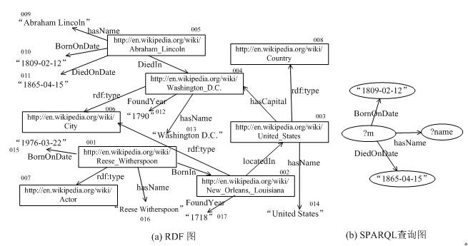
Figure 3: RDF graph and SPARQL query graph
2
Current Applications of Knowledge Graphs
This chapter briefly introduces the relevant applications of Knowledge Graphs in the industry, especially in the internet field. In fact, Knowledge Graph technology has seen numerous applications in other fields, including industrial design and product management, knowledge publishing, healthcare, and intelligence analysis. Due to space limitations, we will mainly introduce the products of relevant companies in the internet field.
As mentioned earlier, the popularity of Knowledge Graphs is attributed to Google’s Knowledge Graph project. Google links all internal information resources uniquely by constructing a Knowledge Graph. For example, “Yao Ming” is an entity in the Knowledge Graph, containing some related attributes such as birth date, location, and height. At the same time, documents and images related to “Yao Ming” crawled by the search engine can also be associated with this entity. The earliest application of Google’s Knowledge Graph project was to provide “knowledge cards” in the search engine results. In traditional search engine result interfaces, a list of documents matching the query term is usually returned, as shown on the left side of Figure 4. However, in Google’s search engine results after May 16, 2012, if the query term matches an entity in Google’s Knowledge Graph, Google will also return some properties of this entity and its relationships in the form of a knowledge card. For example, when we search for “Yao Ming”, Google will return a knowledge card on the right side of Figure 4, including Yao Ming’s birth date, location, height, and his wife Ye Li; it may even include related images of Yao Ming.

Figure 4: Knowledge card in Google search results
Next, we introduce another project by Google that utilizes Knowledge Graphs called “Google Rich Snippets”. The search engine provides a summary of the target webpage for each search result, allowing users to judge whether it is the page they want to search for. Typically, webpage summaries are generated using an “extraction” method, which finds important sentences related to the search keywords from the webpage text to form the summary returned to users. However, in Google’s Rich Snippets product, knowledge graph data that exists in a structured form in the user’s HTML page is extracted, such as data describing the attributes of entities. Currently, standards for this area include structured data tags like RDFa, Microdata, and Schema.org. Suppose a user wants to search for the product “Thinkpad T450”; in the summary of the Walmart online store page returned by Google (as shown in Figure 7), the summary includes the product rating (Rating 3 stars), number of reviews (Vote 1 review), and product price ($616.67). In fact, this important data has already been marked in the HTML by the user through structured semantic tags like Schema.org, allowing the search engine to parse this structured data and use this structured knowledge graph data to generate the summary. We show in Figure 6 how to extract the aforementioned product price and brand attributes from the Walmart product page’s HTML using Google’s structured testing tool.

Figure 5: A product page from Walmart online store
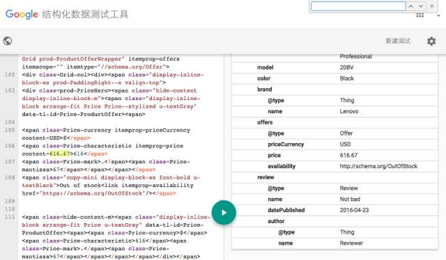
Figure 6: Structured data extracted by Google’s structured extraction tool from the “Walmart product page”
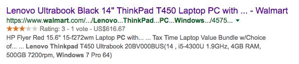
Figure 7: Search result summary of the “Walmart product page” generated based on extracted structured data
Facebook has also defined a similar tagging language called Open Graph Protocol (OGP). Facebook uses the OGP protocol to define the knowledge graph in social networks, known as the Facebook Social Graph, which connects users of the social network, user-shared photos, movies, comments, and even third-party knowledge graph data linked through Facebook’s defined Graph API. Based on the constructed Social Graph, Facebook launched the Graph Search feature. This feature converts users’ natural language questions into graph search queries on the Social Graph to answer users’ questions. For example, if I log in with my Facebook account and input the natural language “My friends who live in Canada”, it will display the accounts of my friends living in Canada; similarly, if I input “Photos of my friends who live in Canada”, it will display the photos shared by these friends on Facebook. This example clearly shows that the Social Graph constructed by Facebook associates users, locations, and photos; otherwise, it would not be able to answer the above two natural language questions. Facebook converts the natural language input into structured query operations on the Social Graph. As shown in Figure 8, the original query statement, after being processed by the natural language interface module, corresponds to the normalized natural language query statement and the structured query statement, which are respectively: “my friends who live in [id:12345]” and “intersect(friends(me), residents(12345))”, where “12345” represents the Facebook ID corresponding to “Canada” in the social graph. The corresponding structured query statement is sent to Facebook’s internally designed index and search system Unicorn, ultimately retrieving the answer.

Figure 8: An example of converting natural language into structured queries in Facebook
Knowledge graph-based question-answering systems also include the EVI product acquired by Amazon. EVI was originally named True Knowledge, a product of a startup. Essentially, it organizes data in the form of triples and uses template technology to convert users’ natural language questions into structured query statements to find results for users. IBM’s Watson system also utilizes DBpedia and Yago knowledge graph data to answer certain natural language questions; compared to traditional document-based question-answering methods, knowledge graph-based question-answering has higher accuracy, but the range of questions it can answer is relatively limited. For example, Figure 9 shows that the coverage of questions that IBM’s Watson system can answer using knowledge graphs is less than the coverage of traditional text search, but the accuracy of question-answering using knowledge graphs is much higher.
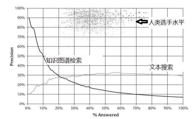
Figure 9: Experimental data from IBM’s Watson system participating in the Jeopardy challenge (excerpted from [3])
3
Data Management Methods for Knowledge Graphs
A core issue in managing knowledge graph data is how to effectively store and query RDF datasets. In general, there are two completely different approaches. One is to utilize existing mature database management systems (e.g., relational database systems) to store knowledge graph data, converting SPARQL queries aimed at RDF knowledge graphs into queries for these mature database management systems, such as SQL queries for relational databases, and using existing relational database products or related technologies to answer these queries. The most critical research issue here is how to construct relational tables to store RDF knowledge graph data and ensure that the converted SQL queries perform better; the second is to directly develop native knowledge graph data storage and query systems (Native RDF graph database systems) that optimize from the bottom up considering the characteristics of RDF knowledge graph management. We will introduce both approaches.
3.1 Methods Based on Relational Data Models
Due to the enormous success of RDBMS (Relational Database Management Systems) in data management and mature commercial software products, and the fact that the RDF triple model can be easily mapped to relational models, many researchers have attempted to design RDF storage and retrieval schemes using relational data models. Depending on the designed table structure, the corresponding storage and query methods vary; below we introduce several classic methods.
-
Simple Triple Table
The simplest method to map RDF data to relational database tables is to create a table with only three columns (Subject, Property, Object), placing all RDF triples in this table. Given a SPARQL query, we design a query rewriting mechanism to convert SPARQL into the corresponding SQL statement, which is answered by the relational database. For example, we can convert the SPARQL query in Figure 2 into the SQL statement shown in Figure 10.
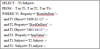
Figure 10: Converted SQL query
Although this method has good generality, the biggest problem is poor query performance. First, the scale of this triple table may be very large; for example, the current DBpedia knowledge base has over 500 million triples. As shown in the SQL statement in Figure 12, there are multiple self-join operations on the tables, which will severely impact query performance.
-
Horizontal Storage
The horizontal method mentioned in the literature is to represent each RDF subject as a row in the database table. The columns in the table include all attributes in the RDF dataset. The advantage of this strategy is its simple design and ease of answering queries aimed at a single subject’s attribute values, known as star queries, as shown in Figure 11.
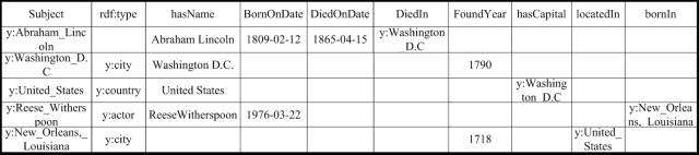
Figure 11: Horizontal storage
According to the table structure shown in Figure 13, to answer the SPARQL query in Figure 2, we can convert it to the following SQL statement. Compared to Figure 12, the SQL statement below does not involve time-consuming join operations, thus its query efficiency is much higher than that of the SQL statement in Figure 12.
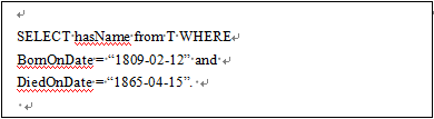
Figure 12: SQL query on horizontal storage
However, this horizontal storage method also has obvious drawbacks: first, there are a large number of columns in the table. Generally speaking, the number of attributes will be much less than the number of subjects and attribute values, but it may still exceed the current database’s handling capacity. Second, there is the sparsity issue of the table. Typically, a subject does not have values for all attributes. Instead, a subject may only have values for a few attributes. However, since a subject is stored as a row, there will be many empty values in the table. Empty values not only increase storage load but also bring other problems, such as increasing index size and impacting query efficiency; the literature has detailed the issues caused by empty values. Third, horizontal storage has the problem of multi-value attributes. The number of columns in a table is fixed, which means a subject can only have one value for an attribute. However, real data often does not conform to this limitation. Fourth, changes in data may incur significant update costs. In practical applications, data updates may lead to the addition or deletion of attributes, which involves changes to the entire table structure, making it difficult for horizontal structures to handle such issues.
-
Attribute Table
An attribute table is an optimization of horizontal storage. By classifying different entities based on the set of attributes associated with each entity, each class adopts a database table with a horizontal storage strategy. The attribute table inherits the advantages of horizontal storage while avoiding issues such as excessive column counts in the table by classifying related attributes. In Jena, attribute tables are used to improve the query efficiency of RDF triples. Researchers have proposed two different types of attribute tables: one is called a clustered property table, and the other is called a property-class table.
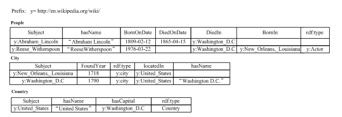
Figure 13: Clustered property table
The clustered property table groups conceptually related attributes into a class, defining a separate database table for each class, and using horizontal storage to store these triples. If some triples do not belong to any category, they are placed in a left-over table. In Figure 13, based on the relevance of attributes, all attributes are clustered into three classes, each class using a horizontal table to store. Similarly, based on the attribute table structure given in Figure 7, we can convert the SPARQL query in Figure 3 into a SQL statement similar to that in Figure 12. The property-class table categorizes all entities by rdf:type, with each class represented by a horizontal table. This organization method requires each entity to have an rdf:type attribute (a label identifying the entity’s classification).
The main advantage of the attribute table is that it can reduce the self-join cost between subjects during queries, thus greatly improving query efficiency. Another advantage of the attribute table is that since attribute values related to an attribute are stored in one column, storage strategies can be designed for that column’s data type to reduce storage space. This avoids the storage inconvenience caused by property values of different data types being stored in one column in the triple storage strategy. Research work in Jena and other studies have proven the effectiveness of attribute tables, but attribute tables also have inherent defects. First, although attribute tables can improve query performance for certain queries, most queries will involve joining or merging multiple tables. For clustered property tables, if the attribute appears as a variable in the query, multiple property tables will be involved; for property-class tables, if the attribute category is not determined in the query, multiple property tables will be involved. In such cases, the advantages of attribute tables become less significant. Second, due to the diverse sources of RDF data, its structural integrity may be poor, leading to weak correlations between attributes and subjects, with similar subjects potentially not containing the same attributes. In this case, the issue of empty values arises. The poorer the structural integrity of the data, the more pronounced the empty value issue becomes.
Third, in reality, a subject may have multiple values for an attribute. In this case, managing these data with RDBMS can be problematic. Among these, the first two issues are interrelated. When the number of columns in a table decreases, the structural requirements become lower, alleviating the empty value problem, but queries will involve more tables; conversely, when the number of columns increases, if the data structure is weak, the empty value problem will become more pronounced.
-
Vertical Partitioning Strategy
Abadi et al. introduced a decomposed storage model (DSM) for semantic web data storage, proposing vertical partitioning technology. Under the vertical partitioning structure, the triple table is rewritten into N tables containing two columns, where N equals the number of attributes in the RDF data. Each table is named after the corresponding attribute, with the first column containing all subjects with attribute values, and the second column containing the values of those attributes for the subjects. The data in each table is sorted by subject, allowing for quick location of specific subjects, and all subject-subject joins can be transformed into efficiently completed sorted merge joins. If storage space is not severely restricted, indexes can also be built on the attribute values in each table or a sorted copy of each table can be created to enhance access performance for specific attribute values and subject-value or value-value joins. Figure 14 shows how to decompose the RDF dataset in Figure 1 into eight binary tables, with each binary table sorted by subject.
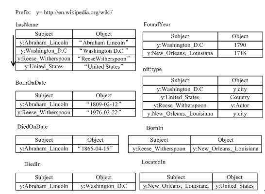
Figure 14: Binary vertical partitioned table
Compared to triple storage, this binary storage method has the following advantages: since attribute names no longer appear repeatedly, it effectively reduces storage space. During queries, only tables related to the query conditions need to be processed, thus effectively reducing I/O costs. Compared to the attribute table method, the advantages of vertical partitioning include the following points. Vertical partitioning is suitable for multi-valued data. Similar to the triple storage method, when a subject has multiple attribute values, it can simply be stored as multiple rows. Vertical storage is also well-suited for poorly structured data; if a subject does not define a certain attribute, that record will not appear in this storage method, avoiding the generation of empty values. Binary storage technology does not require clustering of attributes, eliminating the need to find good clustering algorithms. During queries, if the attribute name is specified, the content of the query will not appear in multiple tables, reducing the need for merge operations. SW-Store utilized vertical partitioning technology and further reduced redundancy in subject storage. However, vertical partitioning technology also has drawbacks. First, this storage method increases the number of join operations. Even if these joins are all low-cost merge joins, the overall computational cost is not negligible. Second, the increased number of tables complicates data updates, especially after SW-Store adopts column storage strategies for space optimization, the system’s update performance faces greater challenges. Updating a subject may involve multiple tables, potentially increasing I/O costs due to external storage methods. When indexes exist on the tables, the update cost becomes even more expensive. Additionally, some literature suggests that storing poorly structured data (such as certain RDF datasets) across multiple tables can lead to issues; reconstructing results returned from multiple tables into a single view may incur high costs.
-
Exhaustive Indexing Strategy
As mentioned earlier, the simple three-column storage method suffers from excessive self-joins. To improve query efficiency for simple three-column storage, a widely accepted method is the “exhaustive indexing” strategy, such as RDF-3X and Hexastore. This method lists all possible permutations of the three-column table (6 types) and establishes clustered B+-trees for each permutation. The benefits of establishing such exhaustive indexes are twofold: first, for each query triple pattern in SPARQL, it can be converted into a range query on a certain permutation. For example, the query triple pattern ?m
Although the exhaustive indexing strategy can compensate for some of the shortcomings of simple vertical storage, there are still many unresolved issues with the triple storage method. First, different triples may have repeated subjects/attributes/attribute values, leading to wasted storage space. Second, complex queries require numerous table join operations; even if well-designed indexes can convert all join operations into merge joins, the query costs for complex SPARQL queries remain non-negligible. Third, as the amount of data grows, the size of the tables will continue to expand, severely degrading system performance; moreover, current systems of this type cannot support distributed storage and querying, limiting their scalability. Fourth, due to the diverse data types, it is challenging to optimize storage based on specific data types, potentially leading to wasted storage space (for instance, the values of objects can vary, such as URIs, general strings, or numbers. The storage space for the objects column must accommodate all possible values, making optimization infeasible). To address this issue, current exhaustive index methods utilize dictionary mapping to map all strings and numbers to independent integer IDs. However, this dictionary mapping method struggles to support SPARQL queries with numerical range constraints and substring constraints in strings.
3.2 Methods Based on Graph Data Models
By viewing RDF triples as labeled edges, RDF knowledge graph data naturally fits the structure of graph models. Therefore, some researchers approach RDF data from the perspective of RDF graph model structure, treating RDF data as a graph and addressing RDF data storage issues through the storage of RDF graph structures. The graph model aligns with the semantic hierarchy of the RDF model, maximizing the retention of semantic information in RDF data, and is conducive to querying semantic information. Additionally, storing RDF data in a graph format allows for leveraging mature graph algorithms and graph databases to design RDF data storage schemes and query algorithms. However, using graph models to design RDF storage and querying also presents challenges. First, compared to ordinary graph models, edges on RDF graphs are labeled and may become query targets; second, typical graph algorithms often have high time complexity, necessitating careful design to reduce real-time query time complexity.
In literature [18], we proposed a method using subgraph matching to answer SPARQL queries and built a related open-source system called gStore. Figure 15 shows the system architecture. During the RDF knowledge graph data import and index construction phase, user-input RDF triple files are first represented as a graph G, which is stored directly using a linked list. To accelerate subgraph matching query speed, we encode each entity node in the RDF graph G along with its neighboring attributes and attribute values into a node with a Bitstring, resulting in a labeled graph G*. We proposed a VS-tree index structure for the G* graph, which effectively supports search space filtering during online query phases. In the query phase, user SPARQL queries are converted into subgraph matching queries, and the results of the subgraph matching queries are used to answer user questions. Figure 16 compares the query performance of the gStore system with that of the widely used RDF knowledge graph storage query systems Virtuoso and Apache Jena on international standard test sets (LUBM and WatDiv) comprising 300 million triples. Since the indexing based on graph structure can consider the overall information of the query graph, generally speaking, the more complex the query graph (for example, the more edges in the query graph), the better the performance of gStore compared to the comparison systems, sometimes achieving performance advantages of an order of magnitude. The distributed version of gStore can manage RDF knowledge graph tasks on a scale of 5-10 billion on a cluster of 10 machines.
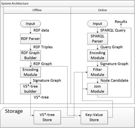
Figure 15: gStore system architecture
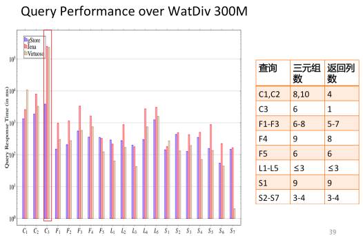
a. Evaluation results on WatDiv dataset with 300 million triples
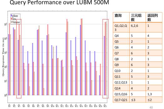
b. Evaluation results on LUBM dataset with 500 million triples
Figure 16: Comparison results on internationally recognized RDF evaluation datasets
Additionally, Udrea et al. proposed the GRIN algorithm to answer SPARQL queries, which is based on constructing a GRIN index similar to an M-tree structure, using distance constraints on the graph to introduce search space. All nodes on the RDF graph are represented as leaf nodes on the GRIN index. Non-leaf nodes on the GRIN index include two elements (center, radius), where center is a central point, and radius is the radius length. Nodes on the RDF graph that are within the shortest path distance from the center that is less than or equal to the radius are descendants of that non-leaf node on the GRIN index. By utilizing distance constraints, GRIN can quickly determine which parts of the RDF graph cannot satisfy the query conditions, thus improving query performance.
Another graph-based system worth mentioning is Trinity.RDF, developed by Microsoft Research Asia, which is a distributed in-memory graph data engine. Due to the poor locality characteristic of graph operations, this system manages RDF graph data using a cloud memory approach. Additionally, to answer subgraph matching queries, Trinity.RDF proposes an exploration strategy on the graph rather than the usual join strategy to find subgraph matching locations.
4
Focus of Knowledge Graph Research in Different Fields
Overall, Knowledge Graphs represent an interdisciplinary research area; different fields of computer science have conducted research on Knowledge Graphs from various perspectives. Figure 16 illustrates this interdisciplinary research situation. The first three chapters mainly introduced the research content of Knowledge Graphs from the perspectives of databases and data management; below, we will briefly introduce the current hot topics in Knowledge Graph research from the fields of natural language processing, knowledge engineering, and machine learning.
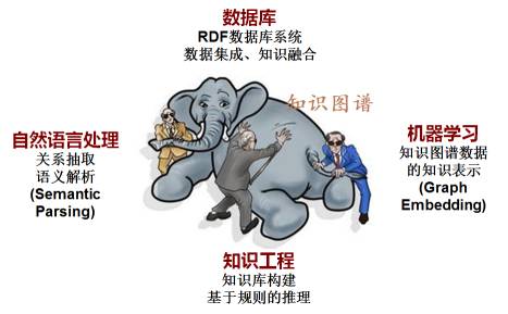
Figure 16: Focus of research on “Knowledge Graph” in different fields
In the field of natural language processing, research on Knowledge Graphs primarily focuses on two aspects. One is “Information Extraction”. Currently, most data on the internet is still “unstructured” text data; how to extract the triple data needed for Knowledge Graphs from unstructured text data is a challenging task. Another very active research topic is “Semantic Parsing”, which involves converting user-input natural language questions into structured queries for Knowledge Graphs.
In the field of knowledge engineering, there are also two main hot research issues. One is the construction of large-scale ontologies and knowledge bases. For example, DBpedia and Yago are both constructed by extracting knowledge from Wikipedia to create large-scale knowledge graph datasets; additionally, the construction of knowledge graphs for specific closed domains is widely applied in the industry. Another research topic is the study of reasoning problems on Knowledge Graphs. It is important to note that Knowledge Graphs differ from traditional databases in that they adopt an open-world assumption. In an open-world assumption, the system does not assume that the stored data is complete; statements that are not explicitly stored in the system but can be inferred are still considered valid data.
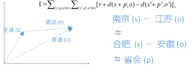
Figure 17: Example of the TransE model
In recent years, the field of machine learning has also seen a surge in research on Knowledge Graphs, with popular topics including “Representation Learning” aimed at Knowledge Graphs, with the most representative research work being the TransE model. Given a knowledge graph, we map each subject, object, and predicate in the knowledge graph triples to a high-dimensional vector, with the optimization objective represented by minimizing the formula in Figure 17. The basic meaning of this formula is that for any triple existing in the knowledge graph G, where the vector representations of the subject, predicate, and object are s, p, and o, respectively, we require that the sum of the vectors of the subject (s) and predicate (p) is as close as possible to the vector representation of the object (o); for triples not present in the knowledge graph G, the distances should be as far apart as possible. Figure 17 visualizes the meaning of the TransE model; the basic idea is that for two triples with the same predicate, the vector differences between their subjects and objects are approximately equal. Based on the TransE model, many improved knowledge graph embedding schemes have been proposed in the academic community. These models have significantly improved accuracy in many tasks, such as predicate prediction and knowledge completion.
5
Conclusion
Knowledge Graph (KG) can be considered, from a certain perspective, as a commercially packaged term; however, it originates from academic research areas such as the semantic web and graph databases. This article attempts to introduce the hot research topics in the field of Knowledge Graphs from the perspective of knowledge data management, as well as the different focuses of various disciplines on Knowledge Graphs. Due to space limitations and the author’s academic research limitations, the introduction of a broader range of Knowledge Graph research and applications inevitably leaves much to be desired, and readers are encouraged to provide criticism and guidance. I, along with my colleagues at the Data Management Research Lab at Peking University, have long been engaged in the area of RDF knowledge graph data management and have developed a graph database system called gStore for managing massive RDF knowledge graph data and a natural language question-answering system called gAnswer. Interested readers can refer to the original papers published on these two systems: VLDB 11 and SIGMOD 14, as well as a recent article summarizing the research ideas of these two Knowledge Graph projects.
(1)http://www.icst.pku.edu.cn/db/en/index.php/Main_Page
(2)http://www.icst.pku.edu.cn/intro/leizou/projects/gStore.htm
(3) http://www.icst.pku.edu.cn/intro/leizou/projects/gAnswer.htm
(4) http://rdcu.be/o1nT
References
[1] https://www.w3.org/TR/sparql11-query/
[2] Michael Curtiss, Iain Becker, Tudor Bosman, Sergey Doroshenko, Lucian Grijincu, Tom Jackson, Sandhya Kunnatur, Søren B. Lassen, Philip Pronin, Sriram Sankar, Guanghao Shen, Gintaras Woss, Chao Yang, Ning Zhang: Unicorn: A System for Searching the Social Graph. PVLDB 6(11): 1150-1161 (2013)
[3] David A. Ferrucci, Eric W. Brown, Jennifer Chu-Carroll, James Fan, David Gondek, Aditya Kalyanpur, Adam Lally, J. William Murdock, Eric Nyberg, John M. Prager, Nico Schlaefer, Christopher A. Welty:
Building Watson: An Overview of the DeepQA Project. AI Magazine 31(3): 59-79 (2010)
[4] RDF Access to Relational Databases. http://www.w3.org/2003/01/21-RDF-RDB-access/
[5]W3C Semantic Web Advanced Development for Europe (SWAD-Europe). http://www.w3.org/2001/sw/Europe/reports/scalable_rdbms_mapping_report/
[6] Storing RDF in a relational database. http://infolab.stanford.edu/~melnik/rdf/db.html
[7]Zhengxiang Pan, Jeff Heflin. DLDB: Extending Relational Databases to Support Semantic Web Queries. In Proceedings of PSSS’2003.
[8] Daniel J. Abadi. Column Stores for Wide and Sparse Data. In Proceedings of CIDR’2007. pp.292~297
[9] Jennifer L. Beckmann, Alan Halverson, Rajasekar Krishnamurthy, Jeffrey F. Naughton. Extending RDBMSs To Support Sparse Datasets Using An Interpreted Attribute Storage Format. In Proceedings of ICDE’2006. pp.58~58
[10] K. Wilkinson. Jena property table implementation. In SSWS. 2006.
[11] Kevin Wilkinson, Craig Sayers, Harumi A. Kuno, Dave Reynolds. Efficient RDF Storage and Retrieval in Jena2. In Proceedings of SWDB’2003. pp.131~150
[12] Daniel J. Abadi, Adam Marcus, Samuel Madden, Kate Hollenbach. SW-Store: a vertically partitioned DBMS for Semantic Web data management. VLDB J., 2009: 385~406
[13] George P. Copeland, Setrag Khoshafian. A Decomposition Storage Model. In Proceedings of SIGMOD Conference’1985. pp.268~279
[14] Jennifer L. Beckmann, Alan Halverson, Rajasekar Krishnamurthy, Jeffrey F. Naughton. Extending RDBMSs To Support Sparse Datasets Using An Interpreted Attribute Storage Format. In Proceedings of ICDE’2006. pp.58~58
[15] Eric Chu, Jennifer L. Beckmann, Jeffrey F. Naughton. The case for a wide-table approach to manage sparse relational data sets. In Proceedings of SIGMOD Conference’2007. pp.821~832
[16] Thomas Neumann, Gerhard Weikum. RDF-3X: a RISC-style engine for RDF. In Proceedings of PVLDB’2008: 647~659
[17] Cathrin Weiss, Panagiotis Karras, Abraham Bernstein. Hexastore: sextuple indexing for semantic web data management. PVLDB, 2008: 1008~1019
[18] Lei Zou, Jinghui Mo, Lei Chen, M. Tamer Özsu, Dongyan Zhao: gStore: Answering SPARQL Queries via Subgraph Matching. PVLDB 4(8): 482-493 (2011)
[19] Octavian Udrea, Andrea Pugliese, V. S. Subrahmanian: GRIN: A Graph Based RDF Index. AAAI 2007: 1465-1470
[20] Kai Zeng, Jiacheng Yang, Haixun Wang, Bin Shao, Zhongyuan Wang: A Distributed Graph Engine for Web Scale RDF Data. PVLDB 6(4): 265-276 (2013)
[21] Paolo Ciaccia, Marco Patella, Pavel Zezula: M-tree: An Efficient Access Method for Similarity Search in Metric Spaces. VLDB 1997: 426-435
[22] Anthony Fader, Stephen Soderland, Oren Etzioni: Identifying Relations for Open Information Extraction. EMNLP 2011: 1535-1545
[23] Percy Liang: Learning executable semantic parsers for natural language understanding. Commun. ACM 59(9): 68-76 (2016)
[24] Jens Lehmann, Robert Isele, Max Jakob, Anja Jentzsch, Dimitris Kontokostas, Pablo N. Mendes, Sebastian Hellmann, Mohamed Morsey, Patrick van Kleef, Sören Auer, Christian Bizer:
DBpedia – A large-scale, multilingual knowledge base extracted from Wikipedia. Semantic Web 6(2): 167-195 (2015)
[25] Thomas Rebele, Fabian M. Suchanek, Johannes Hoffart, Joanna Biega, Erdal Kuzey, Gerhard Weikum: YAGO: A Multilingual Knowledge Base from Wikipedia, Wordnet, and Geonames. International Semantic Web Conference (2) 2016: 177-185
[26] A. Bordes, N. Usunier, A. Garcia-Duran, J. Weston, and O. Yakhnenko. Translating embeddings for modeling multi-relational data. In Advances in Neural Information Processing Systems, pages 2787–2795, 2013
[27] Lei Zou, Ruizhe Huang, Haixun Wang, Jeffrey Xu Yu, Wenqiang He, Dongyan Zhao:
Natural language question answering over RDF: a graph data driven approach. SIGMOD Conference 2014: 313-324
[28] Lei Zou and M. Tamer Özsu. Graph-based RDF Data Management, Data Sci. Eng. (2017). doi:10.1007/s41019-016-0029-6, http://rdcu.be/o1nT (open access link)
[29] William Tunstall-Pedoe: True Knowledge: Open-Domain Question Answering Using Structured Knowledge and Inference. 80-92
[30] Lei Zou, M. Tamer Özsu,Lei Chen, Xuchuan Shen, Ruizhe Huang, Dongyan Zhao. gStore: A Graph-based SPARQL Query Engine. VLDB Journal, VLDB J, 2014.
[31] 段楠,从图谱搜索看搜索技术的发展趋势,中国计算机学会通讯,2013年8月第90期
Author Information

Lei Zou
Associate Professor, Peking University
National Excellent Young Scholar Fund Recipient