

Andrew Ng’s DeepLearning.ai Course Notes
【Andrew Ng’s DeepLearning.ai Notes 1】Intuitive Explanation of Logistic Regression
【Andrew Ng’s DeepLearning.ai Notes 2】Popular Explanation of Neural Networks Part 1
【Andrew Ng’s DeepLearning.ai Notes 2】Popular Explanation of Neural Networks Part 2
Is deep learning not working well? Andrew Ng helps you optimize neural networks (1)
To improve the training efficiency of a deep neural network, one must approach optimization from various aspects, optimizing the entire computation process while preventing various potential issues.
This article covers several gradient descent methods for optimizing deep neural networks, including Momentum, RMSProp, Adam optimization algorithms, learning rate decay, and batch normalization.
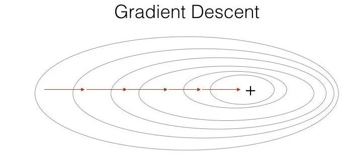
1Batch Gradient Descent (BGD)
Batch Gradient Descent (BGD) is the most commonly used form of gradient descent, which was used in previous logistic regression and deep neural network constructions. It updates parameters using all samples for each update, with the specific process as follows:
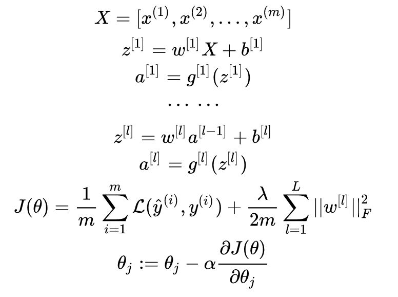
Example image:
-
Advantages: Minimizes the loss function for all training samples, achieving a global optimal solution; easy to implement in parallel.
-
Disadvantages: The training process can be slow when the number of samples is large.
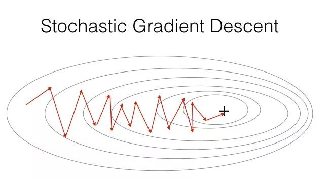
2Stochastic Gradient Descent (SGD)
Stochastic Gradient Descent (SGD) is similar in principle to batch gradient descent, with the difference being that it iteratively updates using one sample at a time. The specific process is as follows:
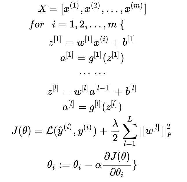
Example image:
-
Advantages: Fast training speed.
-
Disadvantages: Minimizes the loss function for each sample, resulting in the final outcome often being near, but not at, the global optimal solution; not easy to implement in parallel.
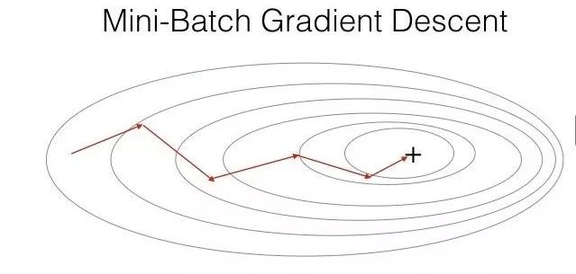
3Mini-Batch Gradient Descent (MBGD)
Mini-Batch Gradient Descent (MBGD) is a compromise between batch gradient descent and stochastic gradient descent, using m training samples, with t (1 < t < m) samples used for iterative updates. The specific process is as follows:
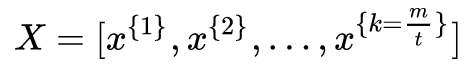
Where,
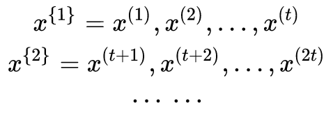
Then,
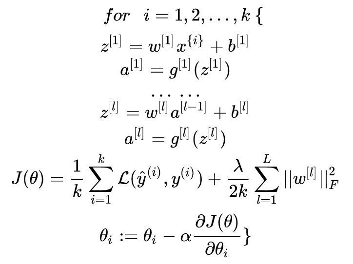
Example image:
The value of the sample size t is adjusted according to the actual number of samples; to adapt to the information storage method of computers, the value of t can be set to a power of 2. Completing one full pass of all training samples is called one epoch.
4Exponential Weighted Average
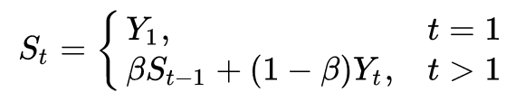
Exponential Weighted Average is a commonly used method for processing sequential data, with the calculation formula as follows:

Given a time series, such as daily temperature values in London for a year:
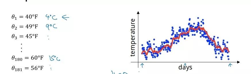
Where the blue points represent the actual data values.
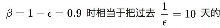
For an instantaneous temperature value, if the weight value β is set to 0.9, then:
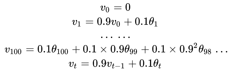
According to:

The value obtained from this is represented by the red curve in the figure, reflecting the general trend of temperature changes.
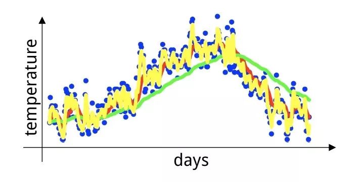
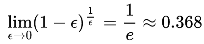
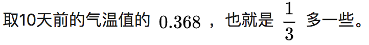
When the weight value β = 0.98, a smoother green curve can be obtained. When the weight value β = 0.5, a yellow curve with more noise is obtained. The larger β is, the more days of averaging are utilized, resulting in a smoother curve that is also more delayed.
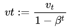
When performing exponential weighted average calculations, the first value ν0 is initialized to 0, which will introduce some bias in early calculations. To correct the bias, the following formula is used after each iteration:
5Momentum Gradient Descent
Gradient Descent with Momentum calculates the exponential weighted average of the gradient and uses this value to update the parameter values. The specific process is as follows:
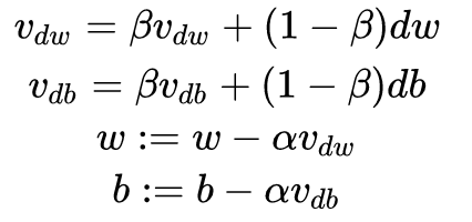
The momentum decay parameter β is generally set to 0.9.
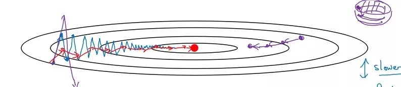
Using standard gradient descent will yield the blue curve in the figure, while using Momentum gradient descent reduces the oscillation along the path to the minimum, accelerating convergence, resulting in the red curve in the figure.
When the gradient directions are consistent, Momentum gradient descent can accelerate learning; when the gradient directions are inconsistent, it can suppress oscillation.
6RMSProp Algorithm
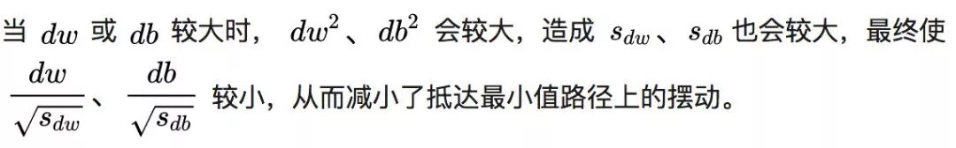
RMSProp (Root Mean Square Prop) algorithm builds on the exponential weighted average of the gradient by introducing squares and square roots. The specific process is as follows:
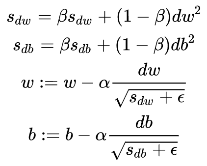
Where ε = 10-8, used to improve numerical stability and prevent the denominator from being too small.
7Adam Optimization Algorithm
Adam (Adaptive Moment Estimation) optimization algorithm is suitable for many different deep learning network structures and essentially combines Momentum gradient descent and RMSProp algorithm. The specific process is as follows:
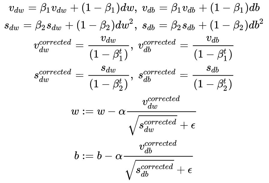
The learning rate α needs to be tuned, with hyperparameter β1 called the first moment, usually set to 0.9, β2 as the second moment, usually set to 0.999, and ε generally set to 10-8.
8Learning Rate Decay
Gradually reduce the learning rate α over time. In the early stages, when α is larger, the steps taken are larger, allowing for faster gradient descent. In the later stages, gradually reducing the value of α decreases the step size, aiding in the algorithm’s convergence and making it easier to approach the optimal solution.
Commonly used learning rate decay methods include:
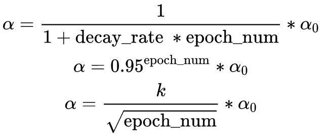
Where decay_rate is the decay rate, and epoch_num is the total number of training epochs.
9Batch Normalization
Batch Normalization (BN) is similar to previous data set normalization and is a method of unifying dispersed data. Uniformly specified data allows machines to learn patterns in the data more easily.
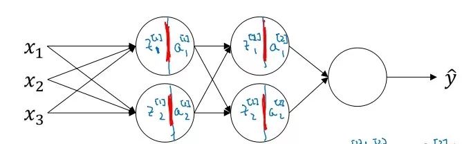
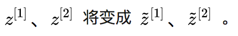
For a layer of a neural network containing m nodes, the steps for performing batch normalization on z are as follows:
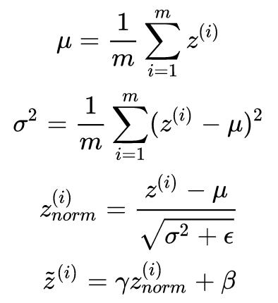
Where γ and β are not hyperparameters but two parameters that need to be learned, allowing the neural network to learn and modify these two scaling parameters. This way, the neural network can gradually determine whether the previous normalization operation has optimized the performance. If not, it can use γ and β to counteract some of the previous normalization operations. For example, when
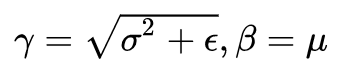
it counteracts the previous regularization operation.

When the current acquired experience cannot adapt to new samples and environments, the “Covariate Shift” phenomenon occurs. For a neural network, the continuous changes in the previous weight values will lead to continuous changes in the subsequent weight values. Batch normalization mitigates the extent of weight distribution changes in the hidden layers. After adopting batch normalization, although each layer’s z continues to change, their mean and variance will remain relatively stable, making the subsequent data and data distribution more stable, reducing the coupling between earlier and later layers, and ultimately accelerating the training of the entire neural network.
Batch normalization also has a regularization effect: when using mini-batch gradient descent, performing batch normalization on each mini-batch introduces some interference to the final z calculated for this mini-batch, producing a regularization effect similar to DropOut, although the effect is not very significant. As the size of the mini-batch increases, the regularization effect weakens.
It is important to note that batch normalization is not a regularization technique; the regularization effect is merely a side effect. Additionally, if batch normalization is used during training, it must also be used during testing.
During training, input is a mini-batch of training samples, while in testing, samples are input one by one. Here, exponential weighted average is utilized again to calculate the weighted average mean and variance for each mini-batch during training, and the final results are saved and applied during testing.
10Softmax Regression
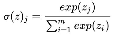
Softmax regression model is an extension of the logistic regression model for multi-class problems. In multi-class problems, the output value y is no longer a single number but a multi-dimensional column vector, with the number of dimensions equal to the number of classes. The activation function used is the softmax function:
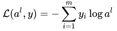
The loss function is:
Note: The images and materials mentioned in this article are compiled and translated from Andrew Ng’s Deep Learning series courses, with all rights reserved. The translation and compilation level is limited; if there are any inaccuracies, please feel free to point them out.

Recommended Reading:
Video | What to Do If You Can’t Write a Paper? Try These Methods
【Deep Learning Practice】How to Handle Variable-Length Sequences Padding in PyTorch
【Basic Theory of Machine Learning】Detailed Explanation of Maximum A Posteriori Estimation (MAP)
Welcome to Follow Our Official Account for Learning and Communication~