302 Page Notes on Andrew Ng’s Deeplearning.ai Course: Key Concepts and Code

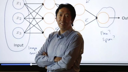
Andrew Ng’s DeepLearning.ai has released its final course on January 31. Recently, Wan Zhen from Chongqing University created a set of notes on the deep learning specialization course, which explains key concepts and assignment codes in detail, starting from the basics of neural networks and deep learning, improving the performance of deep neural networks, and convolutional neural networks. This article provides a summary of the main content of these three courses and highlights interesting knowledge points for each course topic.

• Resource link: https://pan.baidu.com/s/1oAqpmUe Extraction password (invalid)

In these notes, Wan Zhen not only introduces the key knowledge points of each course but also explains the programming assignments in detail. In the first course, “Neural Networks and Deep Learning Basics”, the notes provide basic Python and NumPy operation notes, starting from the basic logistic regression derivation to the most general deep fully connected network. Of course, it also introduces necessary loss functions and backpropagation methods. In the second course, the notes detail the techniques and fundamentals needed to improve deep network performance, such as initialization, regularization, and gradient checking, which greatly enhance model performance in practice, as well as common optimization methods like SGD, momentum, and adaptive learning rate methods. Finally, the second course focuses on TensorFlow, including commonly used functions in the framework and the actual process of building networks. The last chapter mainly records convolutional neural networks, including basic convolution operations, residual networks, and object detection frameworks.

Below is a brief framework of the course notes and some detailed knowledge points.

1. Neural Networks and Deep Learning

This part corresponds to the first lesson of Andrew Ng’s deep learning course, mainly introducing necessary programming languages and programming tools, and gradually progressing from linear networks, nonlinear networks, hidden layer networks to deep network implementation methods, with detailed explanations and complete code. Through this part of study, you will understand the structure and data flow (forward propagation and backward propagation) of neural networks, the role of nonlinear activation functions and hidden layers in learning complex functions, and how to gradually build a complete (arbitrary structure, custom) neural network, experiencing the benefits of vectorized and modular programming concepts.

1.1 Python Basics and Numpy

This chapter’s first section introduces how to use Python’s Numpy toolkit, iPython Notebook, and other basic programming tools. It then explains how to build neural networks with these tools, especially understanding the vectorized idea of neural network computation and the use of Python broadcasting.

1.2 Logistic Regression

The second section introduces how to build a logistic regression neural network classifier (image recognition network) with an accuracy of 70% to recognize cats, and discusses methods to further improve accuracy, as well as the process of updating parameters using the partial derivative of the loss function. It particularly emphasizes using vectorized structures instead of loop structures unless necessary (for example, epoch iterations must use loop structures).

1.2.1 Introduction to necessary Python toolkits; 1.2.2 Introduction to the structure of the dataset; 1.2.3 Overview of the entire learning algorithm’s macro structure; 1.2.4 Introduction to the basic steps of building the algorithm; 1.2.5 and 1.2.6 summarize previous content for code implementation and visual analysis; 1.2.7 Introduction to how to train this neural network with your own dataset; 1.2.8 Complete code of the logistic regression neural network.

Among them, the basic steps for building the algorithm introduced in 1.2.4 are:

• Define model structure;

• Initialize model parameters;

• Loop iteration structure:

• Calculate the current loss function value (forward propagation)

• Calculate the current gradient value (backward propagation)

• Update parameters (gradient descent)

Usually, parts 1-3 are built separately and then integrated into a function model().

1.2.5 Implemented the code for model() and plotted the loss function and gradient graphs.

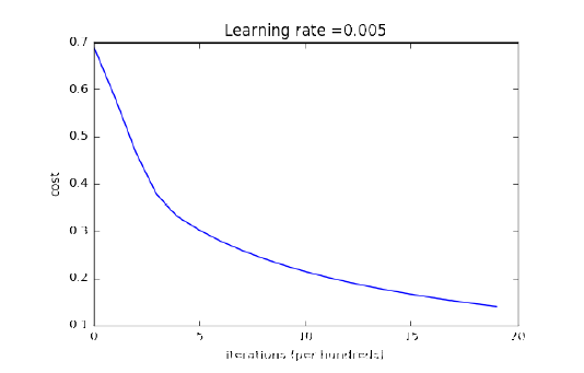
Figure 1.2.3: Loss Function

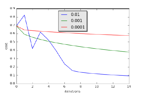
Figure 1.2.4: Comparison of Learning Curves with Three Different Learning Rates

1.3 Classifying Plane Data Points with Hidden Layers

The third section introduces how to add hidden layers to the neural network to classify plane data points. This section will teach you to understand the working process of backpropagation, the role of hidden layers in capturing nonlinear relationships, and how to build auxiliary functions.

Key content includes: implementing a binary classifier with a single hidden layer; using nonlinear activation functions; calculating cross-entropy loss; implementing forward and backward propagation.

1.3.1 Introduction to necessary toolkits; 1.3.2 Introduction to the composition of the dataset (red and blue points on the plane); 1.3.3 Introduction to the classification results of the dataset without hidden layers using logistic regression; 1.3.4 Introduction to the implementation process of the complete model with hidden layers and its classification results on the dataset; 1.3.5 Complete code demonstration.

The classification results used in 1.3.3 are shown in the figure below:

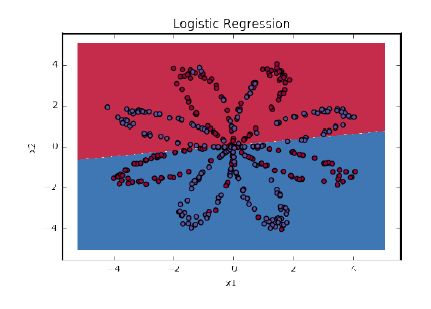
Figure 1.3.3: Logistic Regression

Architecture of the neural network used in 1.3.4:

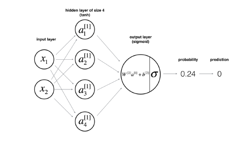
Figure 1.3.4: Neural Network Model

1.3.4 The method of building the neural network is similar to that of 1.2.4, emphasizing how to define the structure of hidden layers and the use of nonlinear activation functions. After implementing the code, the running result is:

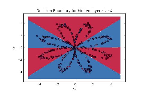
Figure 1.3.6: Decision Boundary of Classifier with Hidden Layer

Among them, after adding hidden layers, it is necessary to use nonlinear activation functions, as stacking linear layers without nonlinear activation functions is meaningless and cannot increase the complexity and capacity of the model.

1.4 Step by Step Building a Complete Deep Neural Network

The fourth section introduces the complete architecture of deep neural networks and how to build custom models. After completing this part, you will learn: using ReLU activation function to enhance model performance, building deeper models (more than one hidden layer), and implementing easy-to-use neural networks (modular thinking).

1.4.1 Introduction to necessary toolkits; 1.4.2 Overview of tasks; 1.4.3 Introduction to the initialization process from 2-layer networks to L-layer networks; 1.4.4 Introduction to the construction of the forward propagation module, from linear forward propagation, linear + nonlinear activation forward propagation, to L-layer network forward propagation; 1.4.5 Introduction to loss functions; 1.4.6 Introduction to the construction of the backward propagation module, from linear backward propagation, linear + nonlinear activation backward propagation, to L-layer network backward propagation; 1.4.7 Complete code of deep neural networks.

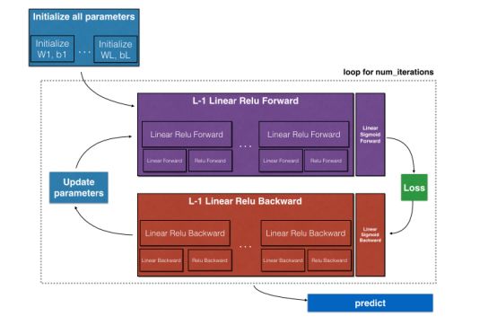
Figure 1.4.1: Task Overview

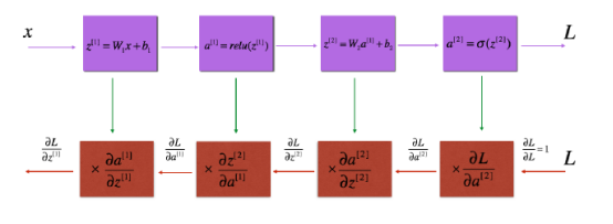
Figure 1.4.3: Illustration of Linear-ReLU-Linear-Sigmoid Process for Forward and Backward Propagation. The top part represents forward propagation, and the bottom part represents backward propagation.

1.5 Image Classification Application of Deep Neural Networks

Through the learning of the previous four sections, you have learned how to build complete deep neural networks step by step. The fifth section introduces how to build a cat recognition classifier using deep neural networks. Previously, the recognition accuracy in the logistic regression network could only reach 68%, while in the complete deep network, the recognition accuracy can reach 80%!

After completing this section, you will learn: how to build neural networks of arbitrary structures using all the auxiliary functions introduced earlier; experiment with different structures of neural networks and analyze them; understand the benefits of building auxiliary functions for constructing networks (compared to starting from scratch).

1.5.1 Introduction to necessary toolkits; 1.5.2 Introduction to the dataset (cats vs. non-cats); 1.5.3 Introduction to model architecture, which builds 2-layer and L-layer neural networks; 1.5.4 Introduction to training and testing results of 2-layer neural networks; 1.5.5 Introduction to training and testing results of L-layer neural networks; 1.5.6 Analysis of results; 1.5.7 Introduction to how to train classification models with your own images; 1.5.8 Complete code demonstration.

Among them, the running results of the 2-layer neural network are:

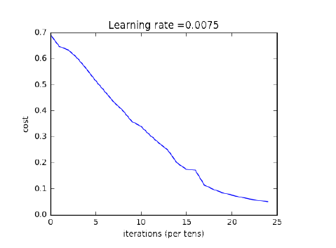
Figure 1.5.4: Loss Function of 2-Layer Neural Network

Running results:

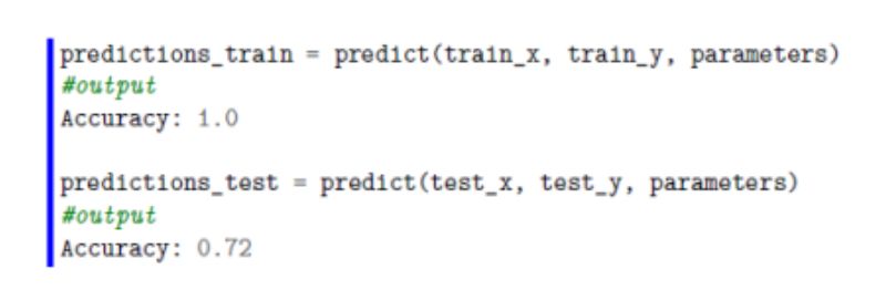
Figure 1.5.5: Loss Function of L-Layer Neural Network

Running results:

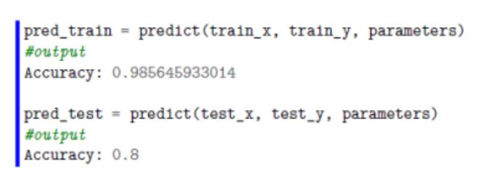
From the comparison, it can be seen that deeper networks help improve recognition accuracy (0.72 vs. 0.8; 2 layers vs. 5 layers).

1.5.6 Briefly summarizes the factors affecting recognition errors:

• Cats appearing in unconventional positions;

• Similar colors of cats and backgrounds;

• Unconventional cat fur colors and breeds;

• Photographing angles;

• Brightness of the photographs;

• Cats occupying too small or too large a proportion of the image.

These recognition errors may be related to the limitations of fully connected networks, including parameter sharing, overfitting tendencies (number of parameters), and hierarchical features, which will be improved in convolutional neural networks.

2. Improving the Performance of Deep Neural Networks

This part corresponds to the second course of Andrew Ng’s deeplearning.ai, focusing on hyperparameter tuning, random and Xavier parameter initialization methods, regularization methods such as Dropout and L2 norm, and gradient checking methods for both 1D and N dimensions to describe practical performance improvement methods in deep learning. Of course, this part not only includes course knowledge points but also showcases Q&A and implementation assignments.

Optimization is also emphasized in this part of the course. Wan Zhen’s notes introduce basic first-order gradient methods from the most basic steepest descent method to mini-batch stochastic gradient descent, and then explore momentum methods and adaptive learning rate methods to utilize historical gradients for better descent directions. Notably, the notes detail the update process and implementation code of the Adam optimization method.

The last part of this course mainly showcases the basic functions of TensorFlow and the actual process of building neural networks.

In parameter initialization, regularization, and gradient checking, the mechanisms of He initialization and Dropout are particularly interesting, and we will explore these two components in detail.

He initialization (He Initialization, He et al., 2015) is named after the first author. If readers are familiar with Xavier initialization, they will find that they are very similar; however, Xavier initialization uses a scalar element sqrt(1./layers_dim[l-1]) for weights W^l, while He initialization uses sqrt(2./layers_dims[l-1]). Below is how to implement He initialization, which is part of the course assignment answer:

# GRADED FUNCTION: initialize_parameters_he
def initialize_parameters_he(layers_dims):
"""
Arguments:
layer_dims -- python array (list) containing the size of each
,→ layer.
Returns:
parameters -- python dictionary containing your parameters "W1",
,→ "b1", ..., "WL", "bL":
W1 -- weight matrix of shape (layers_dims[1],
,→ layers_dims[0])
b1 -- bias vector of shape (layers_dims[1], 1)
...
WL -- weight matrix of shape (layers_dims[L],
,→ layers_dims[L-1])
bL -- bias vector of shape (layers_dims[L], 1)
"""
np.random.seed(3)
parameters = {}
L = len(layers_dims) - 1 # integer representing the number of
,→ layers
for l in range(1, L + 1):
### START CODE HERE ### (
2 lines of code)
parameters['W' + str(l)] = np.random.randn(layers_dims[l],
,→ layers_dims[l-1]) * np.sqrt(2./layers_dims[l-1])
parameters['b' + str(l)] = np.zeros((layers_dims[l], 1))
### END CODE HERE ###
return parameters

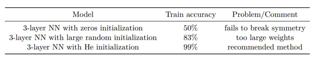
Finally, the document summarizes the effects of three initializations. As shown below, they are tested under the same number of iterations, the same hyperparameters, and the same network architecture:

Dropout

In regularization methods, Dropout is a very useful and successful technique. Although recent researchers have found that using it with batch normalization (BN) may cause some conflicts, it still does not affect its status as a powerful technique to control model overfitting. Generally, Dropout randomly removes some neurons to train different neural network architectures on different batches.

Bagging is a technique that reduces generalization error by combining multiple models. The main approach is to train several different models separately and then let all models vote on the output of the test samples. Dropout can be considered a Bagging method that integrates a large number of deep neural networks, thus providing a cheap Bagging ensemble approximation method that can train and evaluate neural networks equivalent to the number of values in the data.

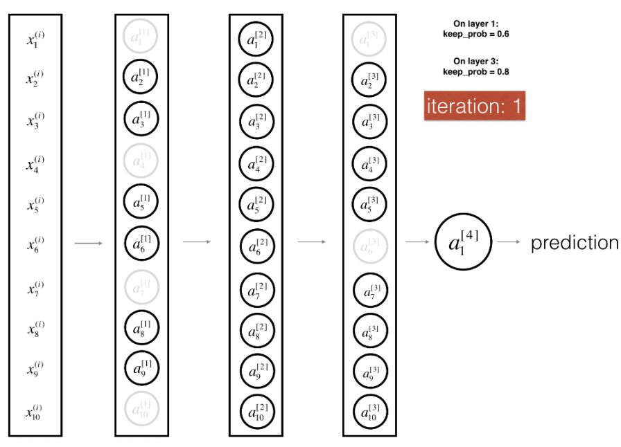
Figure: Using Dropout in the First and Third Layers.

In each batch’s forward propagation and backward updates, we turn off each neuron’s probability of 1-keep_prob, and the turned-off neurons do not participate in forward propagation calculations and parameter updates. Every time we turn off some neurons, we actually modify the original model’s structure, so each iteration trains a different architecture, and parameter updates focus more on activated neurons. This regularization method can be seen as an ensemble method, integrating different network architectures trained in each batch.

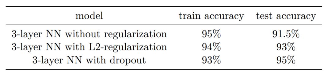
In regularization methods, the effects of L2 regularization and Dropout are also compared:

In the later optimization methods, we are particularly interested in the Adam method, so we will also emphasize this method.

Adam

The Adam algorithm differs from traditional stochastic gradient descent. Stochastic gradient descent maintains a single learning rate (i.e., alpha) to update all weights, and the learning rate does not change during training. In contrast, Adam designs independent adaptive learning rates for different parameters by calculating the first and second moment estimates of the gradients.

The proponents of the Adam algorithm describe it as a combination of the advantages of two extended stochastic gradient descent methods:

• The adaptive gradient algorithm (AdaGrad) retains a learning rate for each parameter to enhance performance on sparse gradients (i.e., natural language and computer vision problems).

• Root Mean Square Propagation (RMSProp) retains adaptive learning rates for each parameter based on the recent magnitudes of weight gradients. This means the algorithm performs excellently on non-stationary and online problems.

The Adam algorithm combines the advantages of both AdaGrad and RMSProp algorithms. Adam not only computes adaptive parameter learning rates based on first moment means like RMSProp, but it also fully utilizes the second moment means of gradients (i.e., biased variance/uncentered variance). Specifically, the algorithm calculates the exponential moving average of the gradients, with hyperparameters beta1 and beta2 controlling the decay rates of these moving averages.

The initial values of moving averages and beta1, beta2 are close to 1 (recommended values), so the bias of moment estimates is close to 0. This bias is improved by first calculating biased estimates and then calculating bias-corrected estimates.

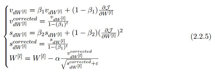
As summarized in the notes, the calculation update process of Adam can be divided into three parts:

1. Calculate the exponentially weighted average of historical gradients and store it in variable v (biased estimate), then calculate v^corrected (corrected unbiased estimate).

2. Calculate the exponentially weighted average of the squares of historical gradients and store it as variable s (biased estimate), then calculate s^corrected (corrected unbiased estimate).

3. Combine the information from the first two steps to update parameters.

This update process can be expressed as follows:

Where t is the number of iterations Adam has updated, L is the number of layers, β_1 and β_1 are hyperparameters controlling the exponential moving averages, α is the learning rate, and ε is a small constant to avoid division by zero.

Wan Zhen also provides the implementation code or assignment interpretation of Adam:

# GRADED FUNCTION: initialize_adam
def initialize_adam(parameters) :
"""
Initializes v and s as two python dictionaries with:
- keys: "dW1", "db1", ..., "dWL", "dbL"
- values: numpy arrays of zeros of the same shape as
,→ the corresponding gradients/parameters.
Arguments:
parameters -- python dictionary containing your parameters.
parameters["W" + str(l)] = Wl
parameters["b" + str(l)] = bl
Returns:
v -- python dictionary that will contain the exponentially weighted
,→ average of the gradient.
v["dW" + str(l)] = ...
v["db" + str(l)] = ...
s -- python dictionary that will contain the exponentially weighted
,→ average of the squared gradient.
s["dW" + str(l)] = ...
s["db" + str(l)] = ...
"""
L = len(parameters) // 2 # number of layers in the neural networks
v = {}
s = {}
# Initialize v, s. Input: "parameters". Outputs: "v, s".
for l in range(L):
### START CODE HERE ### (approx. 4 lines)
v["dW" + str(l+1)] = np.zeros(parameters["W" + str(l+1)].shape)
v["db" + str(l+1)] = np.zeros(parameters["b" + str(l+1)].shape)
s["dW" + str(l+1)] = np.zeros(parameters["W" + str(l+1)].shape)
s["db" + str(l+1)] = np.zeros(parameters["b" + str(l+1)].shape)
### END CODE HERE ###
return v, s

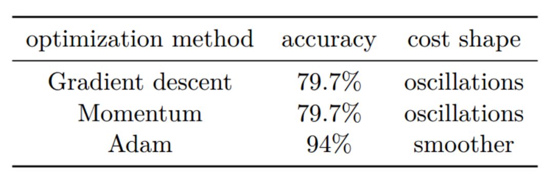
This section also introduces and compares the advantages of these optimization methods:

TensorFlow

The last part focuses on the functions and practices of TensorFlow. TensorFlow is an open-source software library that uses data flow graphs for numerical computation. Here, Tensor represents that the transmitted data is a tensor (multi-dimensional array), and Flow represents performing calculations using the computation graph. The data flow graph is described as a directed graph composed of “nodes” and “edges” to represent mathematical operations. “Nodes” generally represent applied mathematical operations, but can also represent the starting and ending points of data inputs and outputs or the endpoints for reading/writing persistent variables. Edges represent the input/output relationships between nodes. These data edges can transmit multi-dimensional data arrays with dynamically adjustable dimensions, namely tensors.

This part of the notes focuses on testing and implementation code for the course, such as the following simple placeholder:

### START CODE HERE ### (approx. 2 lines)
X = tf.placeholder(tf.float32, [n_x, None], name = 'X')
Y = tf.placeholder(tf.float32, [n_y, None], name = 'Y')
### END CODE HERE ###
return X, Y


return parameters, v, s

Methods for defining variables and constants:

a = tf.constant(2, tf.int16)
b = tf.constant(4, tf.float32)
g = tf.constant(np.zeros(shape=(2,2), dtype=np.float32))

d = tf.Variable(2, tf.int16)
e = tf.Variable(4, tf.float32)

h = tf.zeros([11], tf.int16)
i = tf.ones([2,2], tf.float32)

k = tf.Variable(tf.zeros([2,2], tf.float32))
l = tf.Variable(tf.zeros([5,6,5], tf.float32))


return parameters, v, s

Methods for initializing parameters:

W1 = tf.get_variable("W1", [25,12288], initializer = tf.contrib.layers.xavier_initializer(seed = 1))
b1 = tf.get_variable("b1", [25,1], initializer = tf.zeros_initializer())


return parameters, v, s

Running the computation graph:

a = tf.constant(2, tf.int16)
b = tf.constant(4, tf.float32)

graph = tf.Graph()
with graph.as_default():
   a = tf.Variable(8, tf.float32)
   b = tf.Variable(tf.zeros([2,2], tf.float32))

with tf.Session(graph=graph) as session:
   tf.global_variables_initializer().run()
   print(f)
   print(session.run(a))
   print(session.run(b))

# Output:

>>> <tf.Variable 'Variable_2:0' shape=() dtype=int32_ref>
>>> 8
>>> [[ 0.  0.]
>>>  [ 0.  0.]]


return parameters, v, s

3. Convolutional Neural Networks

In Andrew Ng’s fourth lesson, we learn about Convolutional Neural Networks, and this chapter’s exercises require you to implement a convolution layer and a pooling layer using Numpy, as well as forward and backward propagation. The packages you will use are:

• Numpy: A basic package for scientific computing in Python.

• Matplotlib: For plotting.

Here are the functions you will learn to implement:

1. Convolution functions, including:

• Zero padding

• Convolution window

• Forward convolution

• Backward convolution

2. Pooling functions, including:

• Forward pooling

• Create mask

• Distribute value

• Backward pooling

The first assignment requires you to implement these functions using Numpy, and the next assignment requires you to build a model using TensorFlow functions.

Chapter three discusses convolutional neural networks, pooling layers, and backward propagation of convolutional neural networks. The convolutional neural network section covers zero padding, single-step convolution, and forward convolution networks; the pooling layer section discusses forward pooling; the backward propagation section discusses convolution layer backpropagation and pooling layer backpropagation.

3.1.3 Convolution Networks

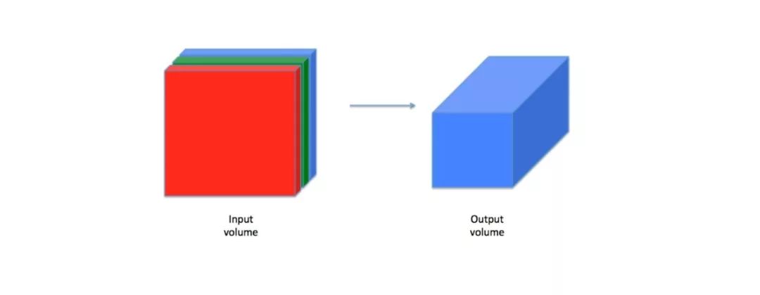
Although programming frameworks make convolution easy to use, convolution remains one of the most difficult parts of deep learning. Convolution networks generally transform inputs into outputs as shown in the figure below:

To help everyone further understand convolution, I will focus on the operation of convolution here.

In this part, we will implement a single-step convolution, which means you perform convolution using a filter at a single position of the input, and the entire convolution result is obtained by continuously moving this filter to every position of the input value. What we need to do:

1: Obtain input data;

2: Perform convolution using the filter at each position of the input data;

3: Output another data (generally of a different size than the input data).

In computer vision, each value in the matrix corresponds to a single pixel value. When we convolve the image with a 3*3 size filter, we multiply each value in the filter by the corresponding value in the original matrix at each position, sum them up, and then add a bias value, and then move this filter to the next position. This is convolution, and the distance moved each time is called the stride. In the first exercise, you will implement a single-step convolution, which is a single real output obtained by convolving the filter at a position of the input data.

Exercise: Implement the conv_single_step() function

Code:

# GRADED FUNCTION: conv_single_step
def conv_single_step(a_slice_prev, W, b):
    """
    Apply one filter defined by parameters W on a single slice
→ (a_slice_prev)oftheoutputactivation
    of the previous layer.
    Arguments:
    a_slice_prev -- slice of input data of shape (f, f, n_C_prev)
    W -- Weight parameters contained in a window - matrix of shape (f,
 → f,n_C_prev)
b -- Bias parameters contained in a window - matrix of shape (1, 1,
 → 1)
Returns:
    Z -- a scalar value, result of convolving the sliding window (W, b)
 → onaslicexoftheinputdata
    """
### START CODE HERE ### (  2 lines of code)
# Element-wise product between a_slice and W. Add bias. s = a_slice_prev * W + b
# Sum over all entries of the volume s
Z = np.sum(s)
### END CODE HERE ###
return Z


return parameters, v, s

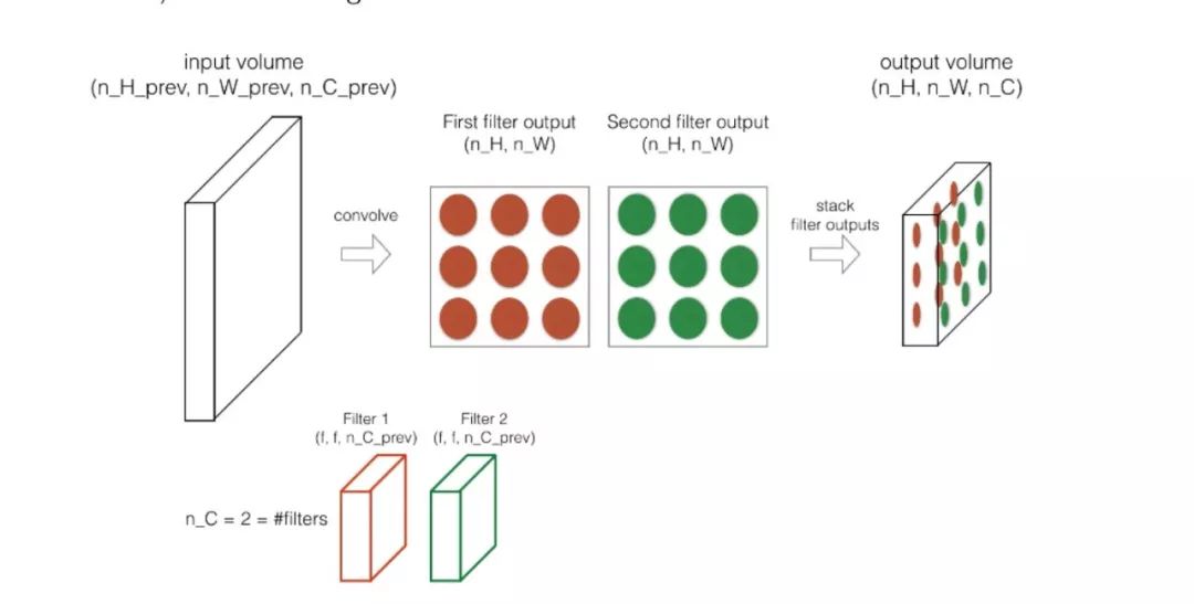
Next, let’s briefly discuss the forward pass of convolutional neural networks. Previously, we discussed how to perform convolution using a filter; in the forward pass, we convolve using multiple filters one by one, and then stack the results (2D) layer by layer into a 3D structure.

For more interesting details, please study Andrew Ng’s course.

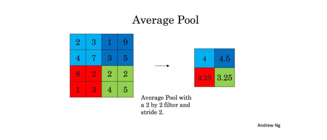
3.1.4 Pooling Layers

Pooling layers are very interesting. To reduce the size of input data and decrease computational load, pooling layers also help feature detectors to be more independent of location information. Here are two types of pooling layers:

• Max pooling layer

Slides a (f,f) size window over the input data, taking the maximum value in the window as output and storing this value in the data prepared for output.

• Average pooling layer

As the name suggests, it similarly slides a (f,f) size window over the input data and calculates the average value of the data in the window, then stores this value in the output.

These pooling layers have no parameters to be trained, but you can try different sizes for the window f and choose the best one.

3.2 Applications of Convolutional Neural Networks

In this section, Andrew discusses TensorFlow models, creating placeholders, initializing parameters, forward propagation, calculating losses, and models.

Let’s talk about how to initialize parameters. You need to use tf.contrib.layers.xavier_initializer(seed=0) to initialize the weights/filters W1 and W2. You don’t need to worry about bias values because you will soon find that TensorFlow functions have already solved this problem. Note that you only need to initialize the weights/filters of the conv2d function; TensorFlow will automatically initialize the fully connected layer parts. We will see more of this in later assignments.

Exercise: Implement initialize_parameters(). The dimensions of each set of filters/weights have been provided for you. Remember, to initialize a parameter W with a shape of [1,2,3,4] in TensorFlow, use:

W = tf.get_variable("W", [1,2,3,4], initializer = ...)

More Info. More information:

# GRADED FUNCTION: initialize_parameters
def initialize_parameters():
"""
Initializes weight parameters to build a neural network with  → tensorflow.Theshapesare:
                        W1 : [4, 4, 3, 8]
                        W2 : [2, 2, 8, 16]
    Returns:
    parameters -- a dictionary of tensors containing W1, W2
    """
tf.set_random_seed(1) # so that your  → "random"numbersmatchours
    ### START CODE HERE ### (approx. 2 lines)
W1 = tf.get_variable("W1", [4, 4, 3, 8], initializer  → =tf.contrib.layers.xavier_initializer(seed=0)) W2 = tf.get_variable("W2", [2, 2, 8, 16], initializer  → =tf.contrib.layers.xavier_initializer(seed=0))
    ### END CODE HERE ###
    parameters = {"W1": W1,
                  "W2": W2}
return parameters

3.3 Keras Tutorial: Happy House

This section discusses an assignment (Happy House), how to build models using Keras, summarize, and test other very useful Keras functions with your own images. Here, let’s focus on what Happy House is:

3.3.1 Happy House

Next time you decide to spend a week with your 5 friends you met at school during your holiday trip. There is a very convenient house nearby where you can do many things. But the most important benefit is that everyone must be happy while in the house. So everyone who wants to enter the room must provide their current happiness level.

As a deep learning expert, to ensure that the “happy” rule is strictly enforced, you need to build an algorithm to check whether a person is happy based on photos taken by the front door camera.

You have collected photos of yourself and your friends taken at the front door, and the database has been labeled. 0 represents unhappy, and 1 represents happy.

Run the following program to standardize the database and then learn about its shape.

X_train_orig, Y_train_orig, X_test_orig, Y_test_orig, classes =  → load_dataset()
# Normalize image vectors
X_train = X_train_orig/255.
X_test = X_test_orig/255.
# Reshape
Y_train = Y_train_orig.T
Y_test = Y_test_orig.T
print ("number of training examples = " + str(X_train.shape[0])) print ("number of test examples = " + str(X_test.shape[0])) print ("X_train shape: " + str(X_train.shape))
print ("Y_train shape: " + str(Y_train.shape))
print ("X_test shape: " + str(X_test.shape)) print ("Y_test shape: " + str(Y_test.shape))
#output
number of training examples = 600
number of test examples = 150
X_train shape: (600, 64, 64, 3)
Y_train shape: (600, 1)
X_test shape: (150, 64, 64, 3)
Y_test shape: (150, 1)

Details of the Happy House database:

• Image data size is (64, 64, 3)

• Training data: 600

• Testing data: 150

Now go solve the “happy” challenge!

3.4 Residual Networks

This section introduces the problems of very deep deep neural networks, how to build residual modules, residual connections, convolution blocks, and how to combine them to build the first residual network model and experiment with your own images.

Residual networks can solve some of the problems associated with very deep deep neural networks, and we will focus on the issues with very deep networks here.

In recent years, neural networks have become increasingly deep, with cutting-edge networks having several layers and even over a hundred layers.

The main advantage of deep neural networks is their ability to represent very complex functions. They can also learn features from different levels of abstraction, from edge features (shallow layers) to complex features (deep layers). However, using a deeper neural network is not always effective. One major drawback is that during model training, gradients can vanish: very deep networks often see their gradients quickly descend to 0. This can make gradient descent unbearably slow, as each update only makes a tiny change. More specifically, during gradient descent, when you backpropagate from the last layer to the first layer, each step involves multiplying by weight matrices, causing gradients to decrease exponentially to 0 (or in some rare cases, the gradients explode exponentially).

During training, you can also observe the gradient values of earlier layers quickly diminishing to 0.

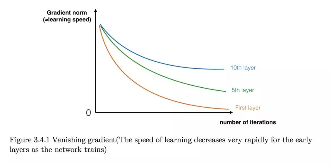
You can now use residual networks to solve this problem.

3.5 Detecting Vehicles with YOLOv2

This section discusses: problem statement, YOLO, model details, filtering scores with a threshold, non-maximum suppression, packaging filters, testing the YOLO model on images, defining classes, breakpoints, and image sizes, loading a trained model, converting output models to usable bounding box tensors, filtering boxes, and running calculations on images.

Here, let’s talk about what the problem is:

You are now working on an autonomous driving car, and as an important part, you want to build a vehicle detection system that will take a look at the road every few seconds while driving.

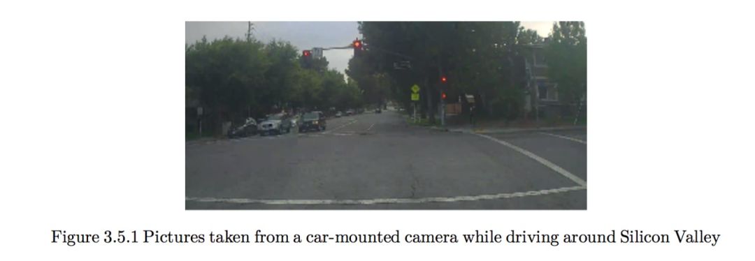
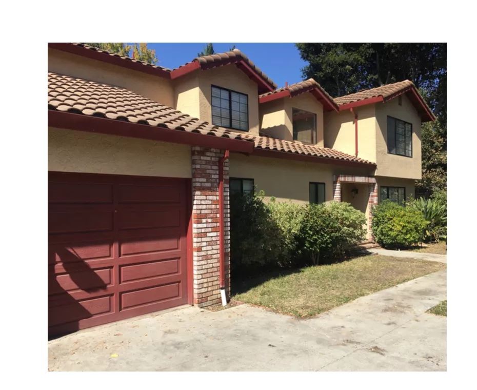
You have already collected all these images into a folder and have annotated each car you can find with boxes. Here is an example:

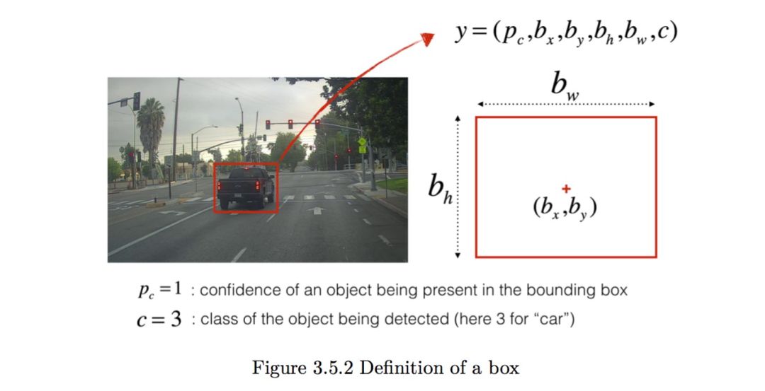
p represents how confident you are in what is circled, and c represents what you think it is.

If you want YOLO to recognize 80 categories, you can let c represent one of the numbers from 1 to 80, or c can be a vector of length 80. The video course has used the latter representation. In this note, we have used both depending on which is more useful. In this exercise, you will learn how YOLO works and how to use it to detect cars. Since training YOLO is very computationally intensive, we will load pre-trained weights for use.

3.6 Face Recognition in the Happy House

In this section, we can see: simplified face recognition, encoding face images into a 128-dimensional vector, using ConvNet for encoding, triplet loss, loading trained models, and using trained models.

Let’s focus on simplified face recognition:

In face recognition, you are given two images and you must tell whether the two individuals are the same person. The simplest approach is to compare each pixel in the two images; if the comparison result of the two original images is below a threshold, you can say the two images are of the same person.

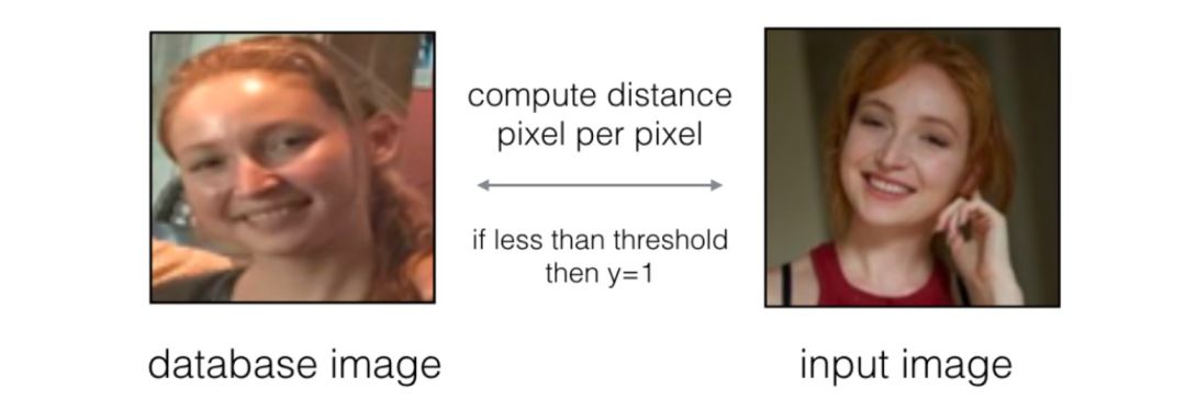
Of course, this algorithm performs very poorly because pixel values can change drastically due to lighting changes, direction changes, or even mirroring head positions. You will see that instead of using the original images, you would prefer to encode f(image) to compare each pixel, which will give you a more accurate answer to whether the two photos are of the same person.

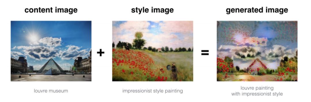
3.7 Generating Art through Neural Style Transfer

In this chapter, we will attempt to implement neural style transfer and use the algorithm to generate novel artistic style images. In neural style transfer, the focus is on optimizing the cost function to obtain pixel values. As shown, we use the style of a certain image and transfer it to an image that needs this style:

Neural style transfer primarily uses pre-trained convolutional neural networks and builds new layers on top of them. This method of using pre-trained models and applying them to new tasks is known as transfer learning. Transfer learning for convolutional networks is very simple; generally, we can randomly initialize the weights of the last few classification layers and quickly achieve excellent performance on new datasets.

In the original paper on NST, we will use the VGG-19 network, which has been pre-trained on ImageNet. Therefore, in Wan Zhen’s notes, we can run the following command to download the model and parameters;

model = load_vgg_model("pretrained-model/imagenet-vgg-verydeep-19.mat")
print(model)

Then use the assign method to set the image as the model’s input:

model["input"].assign(image)

Subsequently, we can use the following code to get the activation values of specific layers:

sess.run(model["conv4_2"])

In neural style transfer, the focus is on the following three steps:

• Construct the content loss function J_content(C, G)

• Construct the style loss function J_style(S, G)

• Combine them into the final loss function J(G) =α J_content(C, G) +β J_style(S, G)

Using such a loss function, we can ultimately achieve neural style transfer through transfer learning.

This article is organized by Machine Heart, please contact the original author for authorization to reprint.

✄————————————————

Join Machine Heart (Full-time Reporter/Intern): [email protected]

Submissions or requests for coverage: [email protected]

Advertising & Business Cooperation: [email protected]