Introduction Want to know how those large-scale neural networks are trained? OpenAI summarizes in an article: Besides needing many GPUs, algorithms are also crucial!
Many advancements in AI today are attributed to large neural networks, especially the pre-trained models provided by large companies and research institutions, which have significantly propelled the progress of downstream tasks.
However, training a large neural network from scratch is not simple. The first challenges include handling massive amounts of data, coordinating multiple machines, and scheduling numerous GPUs.
Mentioning “parallelism” often brings to mind many hidden bugs.
Recently, OpenAI released an article detailing some of the techniques and underlying principles for training large neural networks, completely eliminating your fear of parallelism!
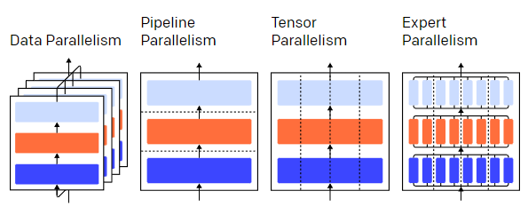
For example, in parallel training of a three-layer neural network, parallelism can be divided into data parallelism, pipeline parallelism, tensor parallelism, and expert parallelism. The different colors in the diagram represent different layers, and the dashed lines separate different GPUs.
It sounds like a lot, but understanding these parallel techniques actually only requires some assumptions about the computational structure and an understanding of the flow direction of data packets.
Training Process Without Parallelism
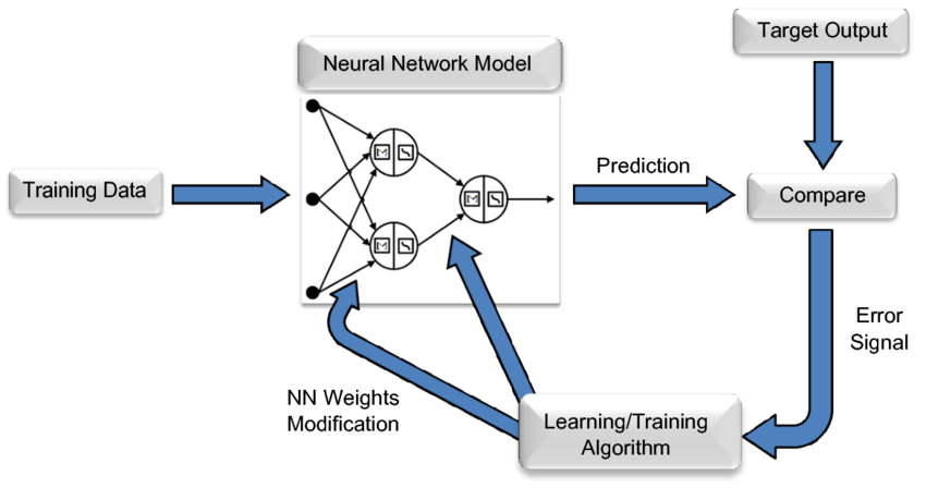
Training a neural network is an iterative process.
In one iteration, input data passes through the layers of the model, and after the forward pass, the output for each training instance in a batch of data can be calculated.
Then, the layers propagate backward, calculating the gradient for each parameter to determine its influence on the final output.
The average gradient for each batch of data, along with parameters and the optimization state for each parameter, is passed to an optimization algorithm, such as Adam, which can compute the next iteration’s parameters (which should perform better on your data) and the new optimization state for each parameter.
As training iterates over massive amounts of data, the model continuously evolves, producing increasingly accurate outputs.
Throughout the training process, various parallel techniques will slice the process across different dimensions, including:
1. Data parallelism, which means running different subsets of a batch on different GPUs;
2. Pipeline parallelism, which means running different layers of the model on different GPUs;
3. Tensor parallelism, which involves splitting a single operation (like matrix multiplication) across different GPUs;
4. Mixture of Experts (MoE), which means using only a portion of each layer to process each input instance.
The GPUs mentioned in parallelism are not limited to GPUs only; these ideas are equally applicable for users of other neural network accelerators.
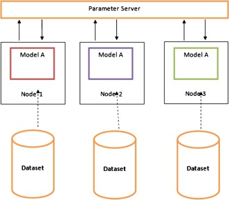
Data parallel training means copying the same parameters to multiple GPUs (often referred to as workers) and assigning different instances to each GPU for simultaneous processing.
Pure data parallelism still requires the model to fit within the memory constraints of a single GPU. If you leverage multiple GPUs for computation, the cost is storing many duplicate copies of parameters. Some strategies can increase the effective RAM available on your GPUs, such as temporarily unloading parameters to CPU memory between uses.
When each data parallel worker updates its parameter copy, they need to coordinate to ensure that each worker continues to have similar parameters.
The simplest method is to introduce blocking communication between workers:
1. Independently compute gradients on each worker;
2. Average gradients across workers;
3. Independently compute the same new parameters on each worker.
Step 2’s blocking requires transferring a significant amount of data (proportional to the number of workers multiplied by the size of the parameters), which can significantly reduce training throughput.
Although various asynchronous synchronization schemes exist to eliminate this overhead, they can compromise learning efficiency; in practice, researchers usually stick to synchronous methods.
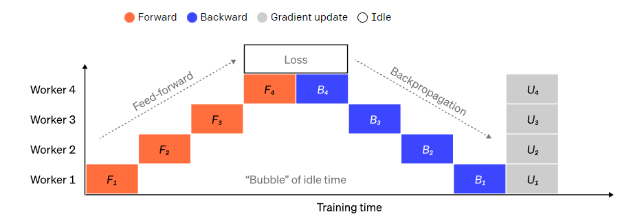
Pipeline parallel training means splitting the sequential blocks of a model across different GPUs, with each GPU holding only a portion of the parameters, thus reducing the memory footprint of the same model on each GPU.
Splitting a large model into large contiguous blocks of layers is a straightforward approach. However, there is a sequential dependency between the inputs and outputs of each layer, so a naive implementation may lead to significant idle time while workers wait for the output of the previous machine to be used as their input.
These waiting time blocks are known as bubbles, wasting computation that idle machines could have completed.
We can reuse the idea of data parallelism by allowing each worker to process only a subset of data elements at a time, cleverly overlapping new computations with waiting times.
The core idea is to split a batch into multiple microbatches; the processing speed of each microbatch should be proportional, with each worker starting work as soon as the next microbatch is available, thereby accelerating pipeline execution.
With enough microbatches, workers remain busy most of the time, and the bubbles at the start and end of each step are minimized. Gradients are averaged across all microbatches, and parameter updates occur only after all microbatches are completed.
The number of workers the model is split into is often referred to as the pipeline depth.
During the forward pass, each worker only needs to send the output (also called activations) of its large block layer to the next worker; during the backward pass, it only sends the gradients of these activations to the previous worker. The scheduling of these transfer processes and how gradients are aggregated in microbatches still has a lot of design space.
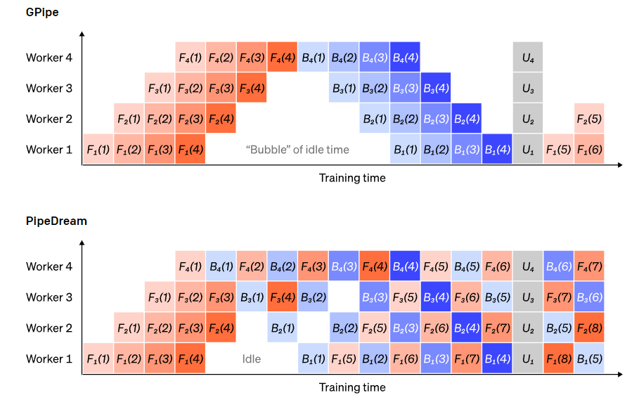
GPipe’s approach is to have each worker continuously process both forward and backward passes, then synchronously aggregate gradients from multiple microbatches at the end. PipeDream, on the other hand, schedules each worker to alternate between processing forward and backward channels.
Pipeline parallelism splits a model “vertically” by layers, while tensor parallelism splits certain operations “horizontally” within a layer.
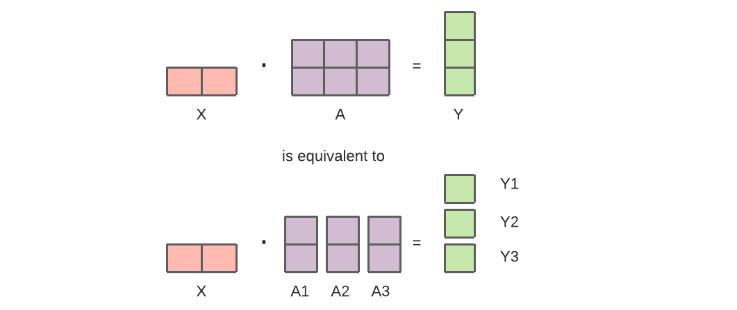
For modern models (like Transformers), the computational bottleneck mainly arises from multiplying the activation batch matrix with large weight matrices. Matrix multiplication can be viewed as the dot product between paired rows and columns, so it is possible to compute dot products independently on different GPUs or compute parts of each dot product on different GPUs, and then sum the results. Regardless of the strategy used, we can slice the weight matrix into even-sized “fragments,” placing each fragment on different GPUs, and using that fragment to compute the relevant part of the entire matrix product, followed by inter-GPU communication to merge the results.
 Megatron-LM adopts this method, parallelizing matrix multiplication within the self-attention and MLP layers of Transformers. PTD-P employs tensor, data, and pipeline parallelism; its pipeline scheduling assigns multiple non-contiguous layers to each device, incurring more network communication at the cost of reducing bubble overhead.
Sometimes, the input to the network can also be parallelized across a dimension, allowing for a high degree of parallel computation relative to cross-communication. Sequence parallelism is such an idea, where an input sequence is split into multiple sub-instances at different times, allowing for proportional reduction of peak memory consumption through finer-grained instance computation.
Megatron-LM adopts this method, parallelizing matrix multiplication within the self-attention and MLP layers of Transformers. PTD-P employs tensor, data, and pipeline parallelism; its pipeline scheduling assigns multiple non-contiguous layers to each device, incurring more network communication at the cost of reducing bubble overhead.
Sometimes, the input to the network can also be parallelized across a dimension, allowing for a high degree of parallel computation relative to cross-communication. Sequence parallelism is such an idea, where an input sequence is split into multiple sub-instances at different times, allowing for proportional reduction of peak memory consumption through finer-grained instance computation.
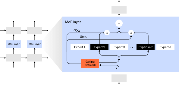
For any input, the MoE strategy only utilizes a portion of the network to compute the output.
For example, a network may have multiple sets of weights, and during inference, the network can use a gating mechanism to select which specific set to use. This allows for an increase in the number of parameters without increasing computational costs.
Each group of weights is referred to as an “expert,” and the training objective is for the network to learn to allocate specialized computations and skills to each expert. Different experts can be hosted on different GPUs, providing a clear method for scaling the number of GPUs used by the model.
GShard can scale the MoE Transformer to 600 billion parameters, where only the MoE layers are split across multiple TPU devices, while other layers remain fully replicated.
Switch Transformer successfully routes an input to an expert, expanding the model’s scale to trillions of parameters, with even higher sparsity.
Besides purchasing GPUs, there are several computational strategies that can help save memory and facilitate training larger neural networks.
1. To compute gradients, you may need to save the original activation values, which can consume a lot of device memory. Checkpointing (also known as activation recomputation) can store any subset of activations and recompute intermediate activations in a just-in-time manner during the backward pass.
This method can save a significant amount of memory, with the computational cost being at most an additional complete forward pass. We can also continuously trade off between computation and memory costs through selective activation recomputation, checking those subsets of activations that have relatively high storage costs but low computational costs.
2. Mixed Precision Training uses lower precision numbers (most commonly FP16) to train the model. Modern computational accelerators can achieve higher FLOPs with low-precision numbers, and you can also save device RAM. If handled properly, this method incurs almost no significant performance loss in the trained model.
3. Offloading is the temporary unloading of unused data to the CPU or different devices, and then reading it back when needed. A naive implementation can significantly reduce training speed, but a complex implementation can pre-fetch data so that devices do not need to wait.
A concrete implementation of this idea is ZeRO, which partitions parameters, gradients, and optimizer states across all available hardware and materializes them as needed.
4. Memory Efficient Optimizers can reduce the memory footprint of the runtime state maintained by the optimizer, such as Adafactor.
5. Compression can also be used to store intermediate results in the network. For example, Gist compresses activations saved for backward passes; DALL-E compresses gradients before synchronizing them.
References:
https://openai.com/blog/techniques-for-training-large-neural-networks/