Neural network algorithms are a type of supervised learning algorithm that can be used to solve classification or regression problems. Their biggest feature is the minimal requirements imposed on the model structure and assumptions, allowing them to approximate various statistical models without needing to assume a specific relationship between the response variable and feature variables in advance. This specific relationship is determined during the learning process. This advantage makes their application very wide-ranging, making them one of the most popular machine learning algorithms today. For example, neural network algorithms can be applied in commercial banks for credit risk assessment of credit customers, scoring credit customers to obtain their probability of default, thereby assessing risks for new or renewed credit business; they can also be applied in real estate customer telemarketing to predict the probability of response to telemarketing, thus enabling more reasonable allocation of marketing resources; in manufacturing, they can predict the purchasing needs of target customer groups to formulate targeted production strategies for cost control. In this chapter, we will explain the basic principles of neural network algorithms and demonstrate their implementation and application in Python for solving classification and regression problems with specific examples.
1. Basic Principles of Neural Network Algorithms
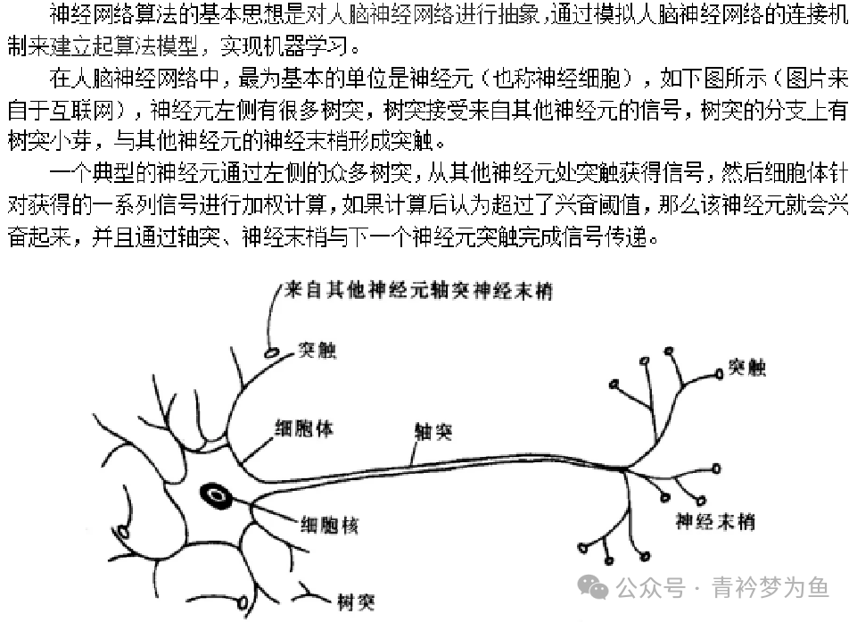
2. Perceptron
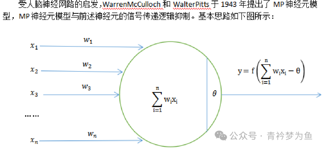
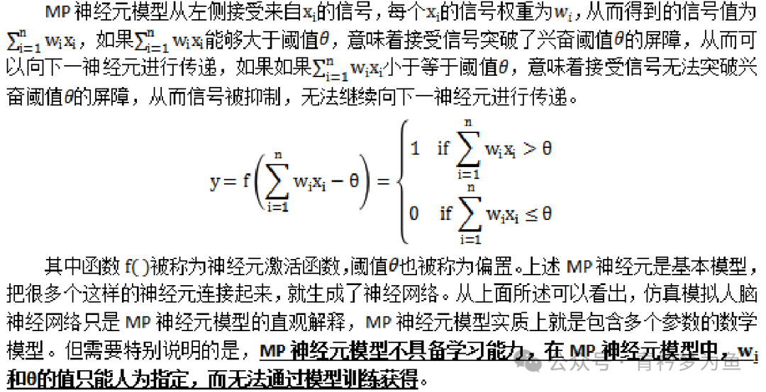
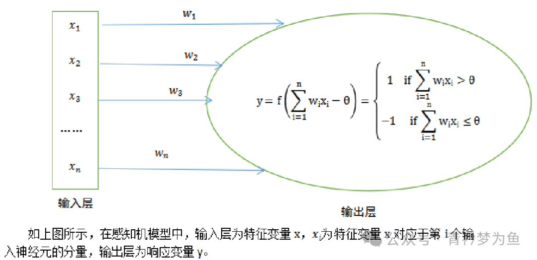
The Perceptron (Perceptron Linear Algorithm, PLA) was proposed by Fran Rosenblatt in 1957. This algorithm enables the MP neuron model to possess learning capabilities and is regarded as the origin of neural networks (deep learning). The basic characteristic of this algorithm is that the model consists of two layers of neurons: the input layer and the output layer, without any hidden layers. The input layer receives external signals, while the output layer is the MP neuron model.


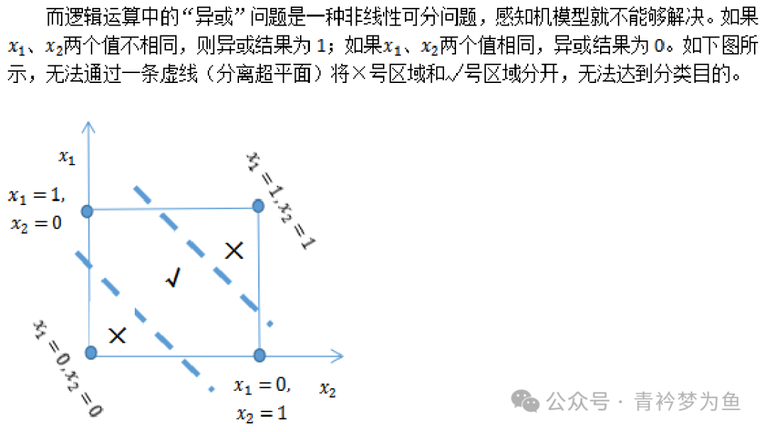
The perceptron cannot solve non-linearly separable problems. To address this issue, we need to extend the two-layer neuron model to more layers, meaning we add hidden layers between the input layer and output layer. Both the hidden layers and output layers can perform substantial data processing through neuron activation functions. For example, a neural network with hidden layers is shown in the figure below.
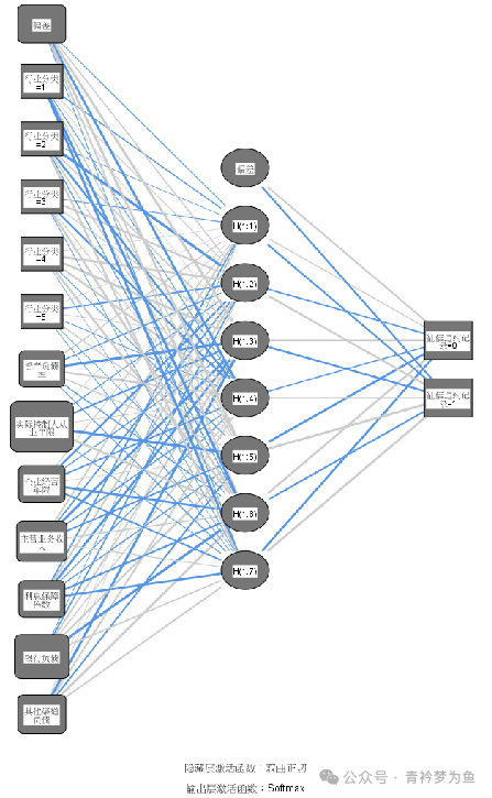
This neural network’s leftmost side is the input layer, including feature variables such as “industry classification”, “debt-to-asset ratio”, “actual controller’s years of service”, “years of business operation”, “main business income”, “interest coverage ratio”, “bank liabilities”, and “other channel liabilities”, without including activation functions; the middle is the hidden layer, which contains unobservable nodes or units, where each hidden unit’s value is the activation function of the feature variables in the “input layer”. The exact form of the function partially depends on the specific type of neural network; in this example, the activation function is the hyperbolic tangent function; on the right side is the output layer’s response variable “credit default record”, where each response is the activation function of the hidden layer; in this example, the activation function is the Softmax function.
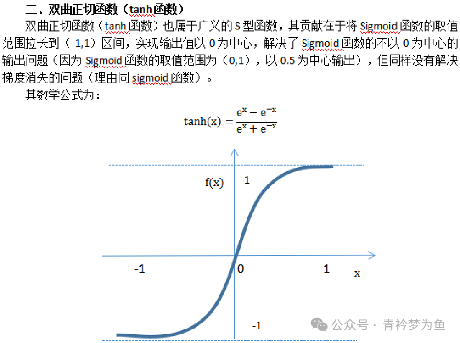
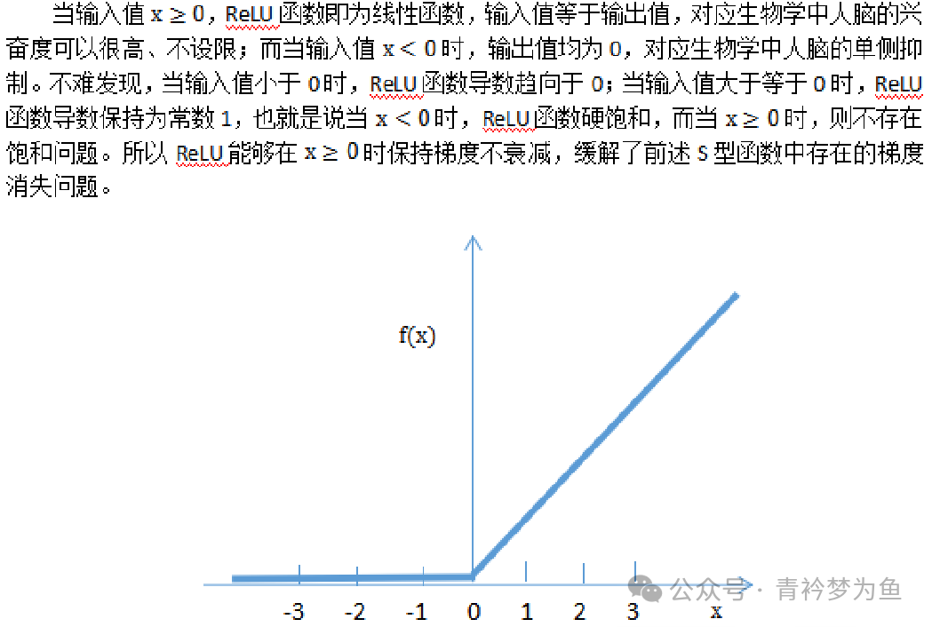
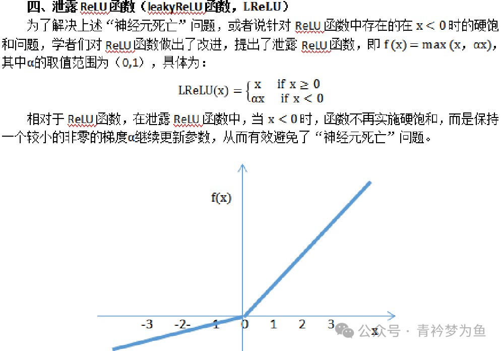
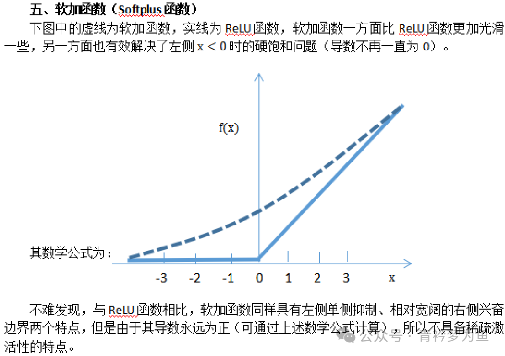
Regardless of the neural network algorithm, its effectiveness is largely due to the existence of activation functions. If we do not set activation functions, then the wisdom of the various layers of the neural network will undergo linear changes based on the neuron connection weight parameters and threshold parameters. Even if we set many hidden layers, the result of linear transformations will still be linear, and it cannot solve any complex non-linear problems. To handle non-linear problems, we need to set activation functions, which must be non-linear. Through the non-linear transformations of activation functions, we can achieve the goal of solving complex learning problems. Commonly used neuron activation functions include: S-shaped function, hyperbolic tangent function, ReLU function, leaky ReLU function, and softplus function.
3. Neuron Activation Functions

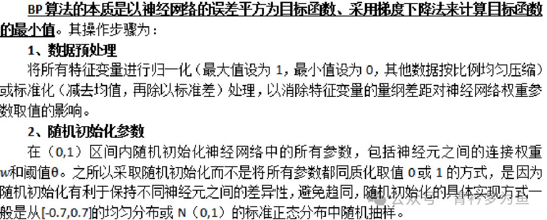
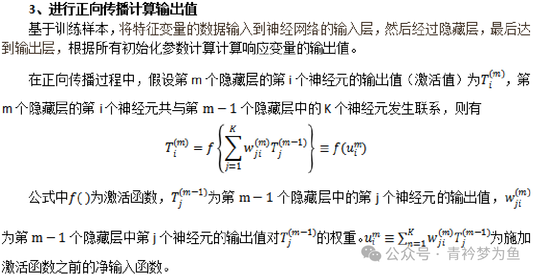
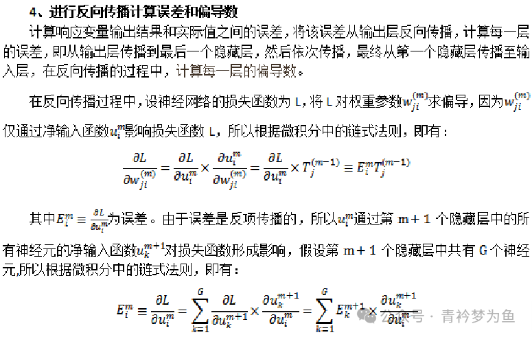
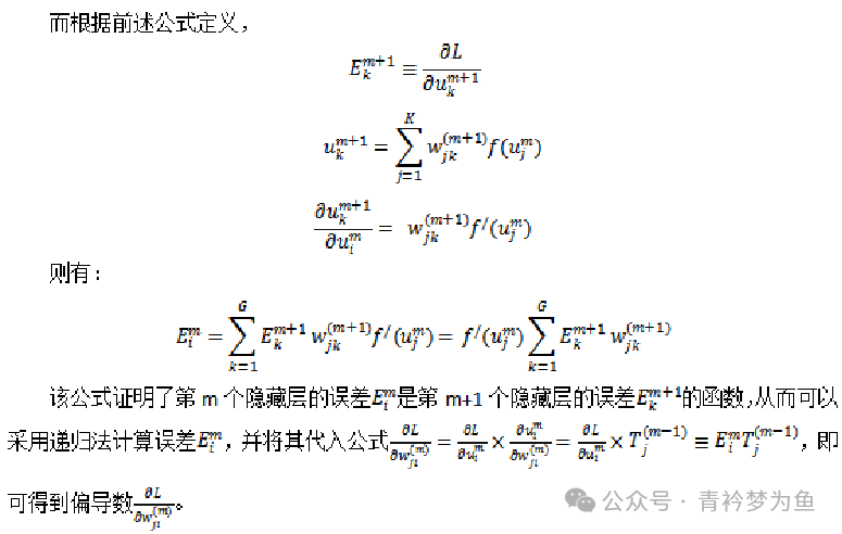
4. Error Backpropagation Algorithm (BP Algorithm)
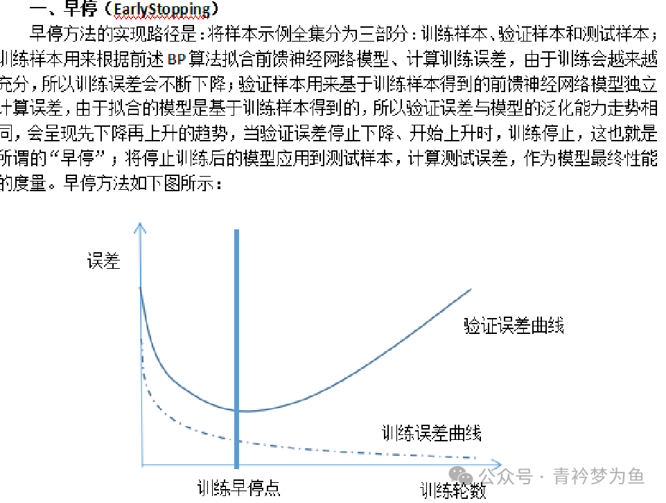
Earlier, we witnessed the power of hidden layers in feedforward neural networks through the BP algorithm and the universal approximation theorem, but it is precisely due to this power that when fitting the model based on training samples, overfitting can easily occur, leading to poor generalization of the model to test samples. To effectively solve this problem, there are two methods to choose from.
Dropout
The dropout method is similar to the idea of bagging; essentially, it trains different networks by randomly hiding neurons, then averages the resulting different neural networks. The implementation path of this method is: during the training of the neural network model based on training samples, some neurons are randomly dropped (or can be understood as temporarily hidden) by randomly setting some neurons’ output values to zero. In other words, these neurons’ subsequent connections are artificially severed, thereby preventing these neurons from transmitting signals outward and affecting the next layer of neurons. During training, parameters of the un-dropped neurons are updated based on the training results, while the parameters of the dropped neurons remain unchanged; in the next training, neurons to be dropped (hidden) are randomly selected again.
Code Example:
import numpy as np
import pandas as pd
import matplotlib
matplotlib.use('TkAgg')
import matplotlib.pyplot as plt
from sklearn.preprocessing import StandardScaler
from sklearn.inspection import permutation_importance
from sklearn.model_selection import train_test_split
from sklearn.neural_network import MLPClassifier
from sklearn.neural_network import MLPRegressor
from sklearn.model_selection import KFold
from sklearn.model_selection import GridSearchCV
from sklearn.inspection import PartialDependenceDisplay
from sklearn.metrics import confusion_matrix
from sklearn.metrics import classification_report
from sklearn.metrics import cohen_kappa_score
from sklearn.metrics import plot_roc_curve
from sklearn.metrics import roc_curve, auc
import matplotlib.pyplot as plt
# Example using plot_roc_curve method
def plot_roc_curve(fpr, tpr, label=None):
plt.figure(figsize=(8, 8))
plt.plot(fpr, tpr, linewidth=2, label=label)
plt.plot([0, 1], [0, 1], 'k--')
plt.axis([0, 1, 0, 1])
plt.xlabel('False Positive Rate')
plt.ylabel('True Positive Rate')
plt.title('ROC Curve')
plt.legend(loc='lower right')
plt.show()
# Then, you can use roc_curve and auc functions to calculate ROC curve parameters
# fpr, tpr, thresholds = roc_curve(true_labels, predicted_scores)
# roc_auc = auc(fpr, tpr)
# Finally, call the custom plot_roc_curve function to plot
# plot_roc_curve(fpr, tpr, label='ROC curve (area = {:.2f})'.format(roc_auc))
# Regression neural network algorithm example
# Variable settings and data processing
data=pd.read_csv('data1.csv')
X = data.iloc[:,1:] # Set feature variables
y = data.iloc[:,0] # Set response variable
X_train, X_test, y_train, y_test = train_test_split(X,y,test_size=0.3, random_state=10)
# Data standardization
scaler = StandardScaler()
scaler.fit(X_train)
X_train_s = scaler.transform(X_train)
X_test_s = scaler.transform(X_test)
X_train_s = pd.DataFrame(X_train_s, columns=X_train.columns)
X_test_s = pd.DataFrame(X_test_s, columns=X_test.columns)
# 17.3.2 Single hidden layer multi-layer perceptron algorithm
model = MLPRegressor(solver='lbfgs', hidden_layer_sizes=(5,), random_state=10, max_iter=3000)
model.fit(X_train_s, y_train)
model.score(X_test_s, y_test)
model.n_iter_
model.intercepts_
model.coefs_
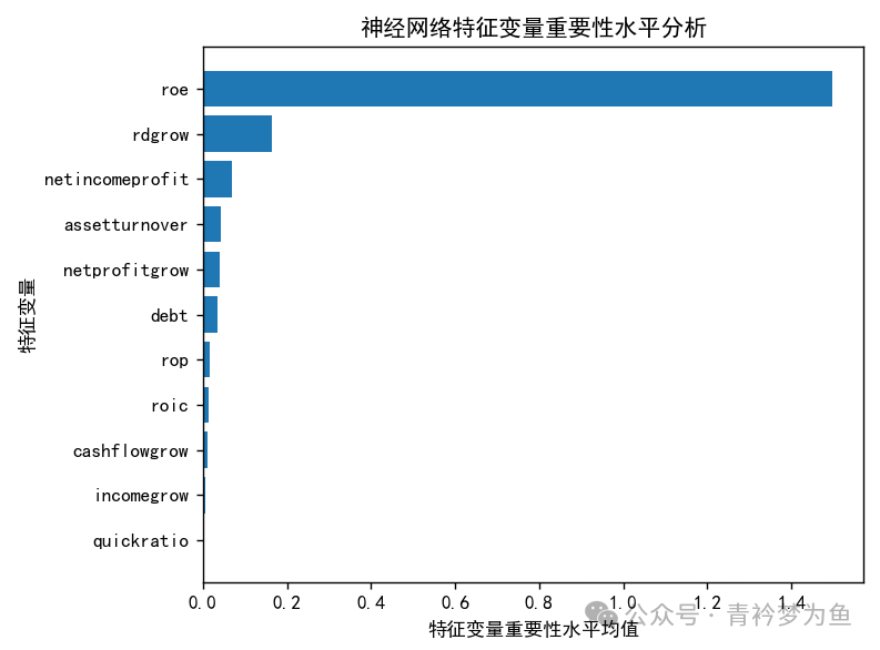
# Neural network feature variable importance level analysis
perm= permutation_importance(model, X_test_s, y_test, n_repeats=10, random_state=10)
dir(perm)
sorted_index = perm.importances_mean.argsort()
plt.rcParams['font.sans-serif'] = ['SimHei'] # Solve Chinese display issues in charts
plt.barh(range(X_train.shape[1]), perm.importances_mean[sorted_index])
plt.yticks(np.arange(X_train.shape[1]), X_train.columns[sorted_index])
plt.xlabel('Feature Variable Importance Mean')
plt.ylabel('Feature Variable')
plt.title('Neural Network Feature Variable Importance Level Analysis')
plt.tight_layout() # Draw partial dependence plots and individual conditional expectation plots
plt.rcParams['axes.unicode_minus']=False # Solve the issue of negative signs not displaying in charts.
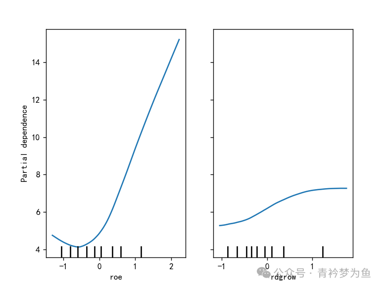
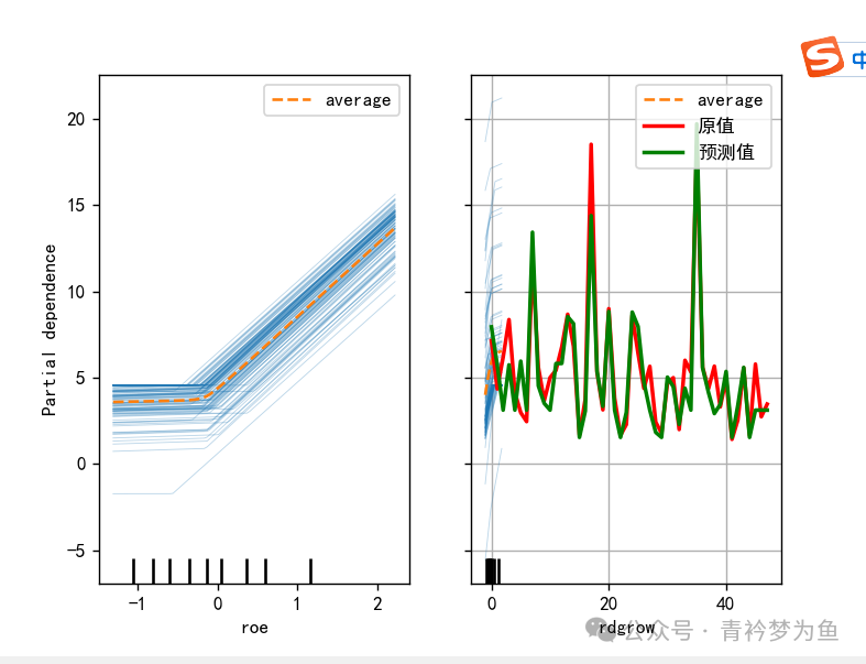
PartialDependenceDisplay.from_estimator(model, X_train_s, ['roe','rdgrow'], kind='average') # Draw partial dependence plot, abbreviated as PDP plot
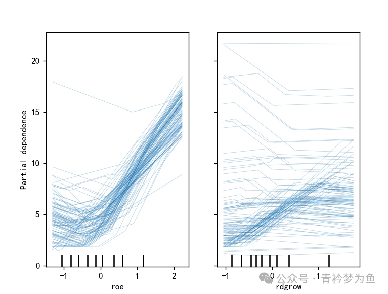
PartialDependenceDisplay.from_estimator(model, X_train_s, ['roe','rdgrow'], kind='individual') # Draw individual conditional expectation plot (ICE Plot)
PartialDependenceDisplay.from_estimator(model, X_train_s, ['roe','rdgrow'], kind='both') # Draw partial dependence plot and individual conditional expectation plot
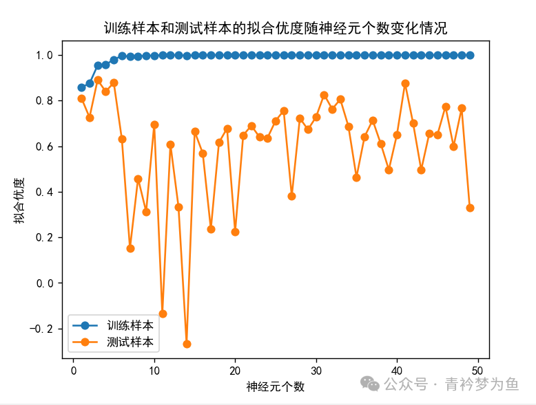
# Visualization of goodness of fit as the number of neurons changes
models = []
for n_neurons in range(1, 50):
model = MLPRegressor(solver='lbfgs', hidden_layer_sizes=(n_neurons,), random_state=10, max_iter=5000)
model.fit(X_train_s, y_train)
models.append(model)
train_scores = [model.score(X_train_s, y_train) for model in models]
test_scores = [model.score(X_test_s, y_test) for model in models]
fig, ax = plt.subplots()
ax.set_xlabel("Number of Neurons")
ax.set_ylabel("Goodness of Fit")
ax.set_title("Goodness of Fit of Training and Testing Samples as the Number of Neurons Changes")
ax.plot(range(1, 50), train_scores, marker='o', label="Training Samples")
ax.plot(range(1, 50), test_scores, marker='o', label="Testing Samples")
ax.legend()
plt.show()
# Seeking the optimal number of neurons in a single hidden layer through K-fold cross-validation
param_grid = {'hidden_layer_sizes':[(1,),(2,),(3,),(4,),(5,),(10,),(15,),(20,)]}
kfold = KFold(n_splits=10, shuffle=True, random_state=1)
model = GridSearchCV(MLPRegressor(solver='lbfgs', random_state=10, max_iter=2000), param_grid, cv=kfold)
model.fit(X_train_s, y_train)
model.best_params_
model = model.best_estimator_
model.score(X_test_s, y_test)
PartialDependenceDisplay.from_estimator(model, X_train_s, ['roe','rdgrow'], kind='average') # Draw partial dependence plot, abbreviated as PDP plot
PartialDependenceDisplay.from_estimator(model, X_train_s, ['roe','rdgrow'], kind='individual') # Draw individual conditional expectation plot (ICE Plot)
PartialDependenceDisplay.from_estimator(model, X_train_s, ['roe','rdgrow'], kind='both') # Draw partial dependence plot and individual conditional expectation plot
# Double hidden layer multi-layer perceptron algorithm
model = MLPRegressor(solver='lbfgs', hidden_layer_sizes=(5, 3), random_state=10, max_iter=3000)
model.fit(X_train_s, y_train)
model.score(X_test_s, y_test)
best_score = 0
best_sizes = (1, 1)
for i in range(1, 5):
for j in range(1, 5):
model = MLPRegressor(solver='lbfgs', hidden_layer_sizes=(i, j), random_state=10, max_iter=2000)
model.fit(X_train_s, y_train)
score = model.score(X_test_s, y_test)
if best_score < score:
best_score = score
best_sizes = (i, j)
best_score
best_sizes
# Visualization of optimal model fitting effect
pred = model.predict(X_test_s) # Predict the response variable
t = np.arange(len(y_test)) # Get the count of the response variable in the test sample for plotting.
plt.rcParams['font.sans-serif'] = ['SimHei'] # Solve Chinese display issues in charts
plt.plot(t, y_test, 'r-', linewidth=2, label=u'Original Value') # Draw the curve of the original value of the response variable.
plt.plot(t, pred, 'g-', linewidth=2, label=u'Predicted Value') # Draw the curve of the predicted value of the response variable.
plt.legend(loc='upper right') # Place the legend in the upper right corner of the chart.
plt.grid()
plt.show()
# Binary classification neural network algorithm example
# Variable settings and data processing
data=pd.read_csv('data13.1.csv')
X = data.iloc[:,1:] # Set feature variables
y = data.iloc[:,0] # Set response variable
X_train, X_test, y_train, y_test = train_test_split(X,y,test_size=0.3, stratify=y, random_state=10)
# Data standardization
scaler = StandardScaler()
scaler.fit(X_train)
X_train_s = scaler.transform(X_train)
X_test_s = scaler.transform(X_test)
X_train_s = pd.DataFrame(X_train_s, columns=X_train.columns)
X_test_s = pd.DataFrame(X_test_s, columns=X_test.columns)
# Single hidden layer binary classification neural network algorithm
model = MLPClassifier(solver='lbfgs', activation='relu', hidden_layer_sizes=(3,), random_state=10, max_iter=2000)
model.fit(X_train_s, y_train)
model.score(X_test_s, y_test)
model.n_iter_
model = MLPClassifier(solver='sgd', learning_rate_init=0.01, learning_rate='constant', tol=0.0001, activation='relu', hidden_layer_sizes=(3,), random_state=10, max_iter=2000)
model.fit(X_train_s, y_train)
model.score(X_test_s, y_test)
# Double hidden layer binary classification neural network algorithm
model = MLPClassifier(solver='lbfgs', activation='relu', hidden_layer_sizes=(3, 2), random_state=10, max_iter=2000)
model.fit(X_train_s, y_train)
model.score(X_test_s, y_test)
model.n_iter_
# Early stopping strategy to reduce overfitting issues
model = MLPClassifier(solver='adam', activation='relu', hidden_layer_sizes=(20, 20), random_state=10, early_stopping=True, validation_fraction=0.25, max_iter=2000)
model.fit(X_train_s, y_train)
model.score(X_test_s, y_test)
model.n_iter_
# Regularization (weight decay) strategy to reduce overfitting issues
model = MLPClassifier(solver='adam', activation='relu', hidden_layer_sizes=(20, 20), random_state=10, alpha=0.1, max_iter=2000)
model.fit(X_train_s, y_train)
model.score(X_test_s, y_test)
model.n_iter_
model = MLPClassifier(solver='adam', activation='relu', hidden_layer_sizes=(20, 20), random_state=10, alpha=1, max_iter=2000)
model.fit(X_train_s, y_train)
model.score(X_test_s, y_test)
model.n_iter_
model = MLPClassifier(solver='adam', activation='relu', hidden_layer_sizes=(20, 20), random_state=10, alpha=0.001, max_iter=2000)
model.fit(X_train_s, y_train)
model.score(X_test_s, y_test)
# Model performance evaluation
np.set_printoptions(suppress=True) # Display numbers directly instead of in scientific notation
prob = model.predict_proba(X_test_s)
prob[:5]
pred = model.predict(X_test_s)
pred[:5]
print(confusion_matrix(y_test, pred))
print(classification_report(y_test, pred))
cohen_kappa_score(y_test, pred) # Calculate kappa score
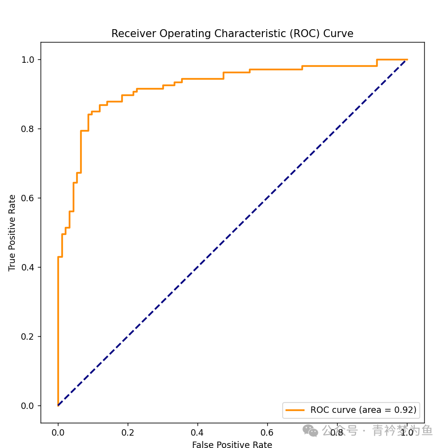
# Draw ROC curve
plt.rcParams['font.sans-serif'] = ['SimHei'] # Solve Chinese display issues in charts
plot_roc_curve(model, X_test_s, y_test)
x = np.linspace(0, 1, 100)
plt.plot(x, x, 'k--', linewidth=1)
plt.title('ROC Curve for Binary Classification Neural Network Algorithm') # Set title to 'ROC Curve for Binary Classification Neural Network Algorithm'
# Using two feature variables to draw the decision boundary plot for the binary classification neural network algorithm
X2_test_s = X_test_s.iloc[:, [2, 5]] # Only select workyears and debtratio as feature variables
model = MLPClassifier(solver='adam', activation='relu', hidden_layer_sizes=(20, 20), random_state=10, alpha=0.1, max_iter=2000)
model.fit(X2_test_s, y_test)
model.score(X2_test_s, y_test)
plot_decision_regions(np.array(X2_test_s), np.array(y_test), model)
plt.xlabel('debtratio') # Set x-axis to 'debtratio'
plt.ylabel('workyears') # Set y-axis to 'workyears'
plt.title('Decision Boundary for Binary Classification Neural Network Algorithm') # Set title to 'Decision Boundary for Binary Classification Neural Network Algorithm'
# Multi-class neural network algorithm example
# Variable settings and data processing
# Variable settings and data processing
data=pd.read_csv('data15.2.csv')
X = data.iloc[:,1:] # Set feature variables
y = data.iloc[:,0] # Set response variable
X_train, X_test, y_train, y_test = train_test_split(X,y,test_size=0.3, stratify=y, random_state=10)
# Data standardization
scaler = StandardScaler()
scaler.fit(X_train)
X_train_s = scaler.transform(X_train)
X_test_s = scaler.transform(X_test)
X_train_s = pd.DataFrame(X_train_s, columns=X_train.columns)
X_test_s = pd.DataFrame(X_test_s, columns=X_test.columns)
# Single hidden layer multi-class neural network algorithm
model = MLPClassifier(solver='sgd', learning_rate_init=0.01, learning_rate='constant', tol=0.0001, activation='relu', hidden_layer_sizes=(3,), random_state=10, max_iter=2000)
model.fit(X_train_s, y_train)
model.score(X_test_s, y_test)
# Double hidden layer multi-class neural network algorithm
model = MLPClassifier(solver='sgd', learning_rate_init=0.01, learning_rate='constant', tol=0.0001, activation='relu', hidden_layer_sizes=(3, 2), random_state=10, max_iter=2000)
model.fit(X_train_s, y_train)
model.score(X_test_s, y_test)
# Model performance evaluation
np.set_printoptions(suppress=True) # Display numbers directly instead of in scientific notation
pred = model.predict(X_test_s)
pred[:5]
print(confusion_matrix(y_test, pred))
print(classification_report(y_test, pred))
cohen_kappa_score(y_test, pred) # Calculate kappa score
# Using two feature variables to draw the decision boundary plot for the multi-class neural network algorithm
X2_train_s = X_train_s.iloc[:, [3, 5]] # Only select income and consume as feature variables
X2_test_s = X_test_s.iloc[:, [3, 5]] # Only select income and consume as feature variables
model = MLPClassifier(solver='sgd', learning_rate_init=0.01, learning_rate='constant', tol=0.0001, activation='relu', hidden_layer_sizes=(3, 2), random_state=10, max_iter=2000)
model.fit(X2_train_s, y_train)
model.score(X2_test_s, y_test) # The running result is 0.8557377049180328.
plt.rcParams['font.sans-serif']=['SimHei'] # Solve Chinese display issues in charts
plt.rcParams['axes.unicode_minus']=False # Solve the issue of negative signs not displaying in charts.
plot_decision_regions(np.array(X2_test_s), np.array(y_test), model)
plt.xlabel('income') # Set x-axis to 'income'
plt.ylabel('consume') # Set y-axis to 'consume'
plt.title('Decision Boundary for Multi-class Neural Network Algorithm') # Set title to 'Decision Boundary for Multi-class Neural Network Algorithm'