Neural Network Algorithms: Introduction and Applications

Implementation Method: Building Basic Module – Neuron

Before discussing neural networks, let’s talk about neurons, which are the basic units of neural networks. Neurons first receive input, perform some mathematical operations, and then produce an output. For the introductory concepts of neural networks, some related understanding concepts are crucial: backpropagation, activation function, and regularization. For example, consider a neuron with 2 inputs:

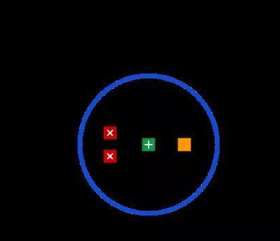
In this neuron, the inputs undergo 3 steps of mathematical operations:

First, multiply the two inputs by weights:

x1→x1 × w1

x2→x2 × w2

Add the two results together, then add a bias:

(x1 × w1) + (x2 × w2) + b

Finally, process them through an activation function to obtain the output:

y = f(x1 × w1 + x2 × w2 + b)

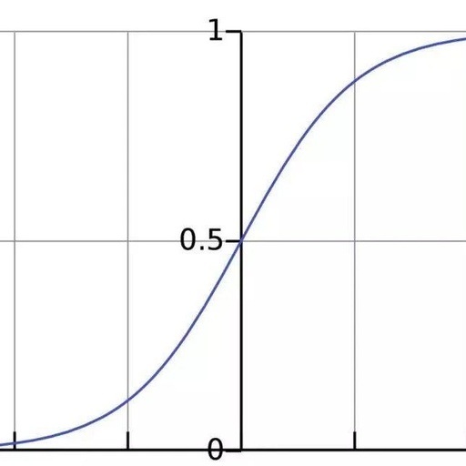
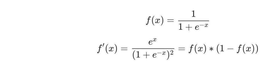
The activation function serves to convert unrestricted inputs into predictable outputs. A commonly used activation function is the sigmoid function:

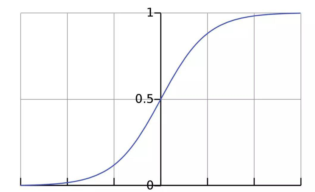
The output of the sigmoid function ranges between 0 and 1, which we can understand as compressing numbers within the range (−∞,+∞) to (0, 1). The larger the positive value, the closer the output approaches 1; the larger the negative value, the closer the output approaches 0.

For example, let’s take the weights and bias in the above neuron as follows:

w=[0,1]

b = 4

w=[0,1] is the vector form of w1=0, w2=1. Given an input x=[2,3], we can compute the output of the neuron using the dot product:

w·x+b = (x1 × w1) + (x2 × w2) + b = 0×2 + 1×3 + 4 = 7

y=f(w⋅X+b)=f(7)=0.999

The Python code for the above steps is:

import numpy as np

def sigmoid(x):

# Our activation function: f(x) = 1 / (1 + e^(-x))

return 1 / (1 + np.exp(-x))

class Neuron:

def __init__(self, weights, bias):

self.weights = weights

self.bias = bias

def feedforward(self, inputs):

# Weight inputs, add bias, then use the activation function

total = np.dot(self.weights, inputs) + self.bias

return sigmoid(total)

weights = np.array([0, 1]) # w1 = 0, w2 = 1

bias = 4 # b = 4

n = Neuron(weights, bias)

x = np.array([2, 3]) # x1 = 2, x2 = 3

print(n.feedforward(x)) # 0.9990889488055994

We called a powerful Python math library called NumPy in the code.

Building a Neural Network

A neural network is formed by connecting a bunch of neurons. Below is a simple example of a neural network:

This network has 2 inputs, a hidden layer with 2 neurons (h1 and h2), and an output layer with 1 neuron (o1). (For this network, the output layer is o1 and o2, and the purpose of backpropagation is to update each w value based on the derivatives so that the new output results o1 and o2 can get closer to the given values, which is the training process.)

The hidden layer is the part sandwiched between the input layer and the output layer, and a neural network can have multiple hidden layers.

The process of passing the inputs of the neurons forward to obtain the outputs is called feedforward.

Assuming all neurons in the above network have the same weights w=[0,1] and bias b=0, and all activation functions are sigmoid, what output will we get?

h1=h2=f(w⋅x+b)=f((0×2)+(1×3)+0)

=f(3)

=0.9526

o1=f(w⋅[h1,h2]+b)=f((0∗h1)+(1∗h2)+0)

=f(0.9526)

=0.7216

The implementation code is as follows:

import numpy as np

# … code from previous section here

class OurNeuralNetwork:

”’

A neural network with:

– 2 inputs

– a hidden layer with 2 neurons (h1, h2)

– an output layer with 1 neuron (o1)

Each neuron has the same weights and bias:

– w = [0, 1]

– b = 0

”’

def __init__(self):

weights = np.array([0, 1])

bias = 0

# The Neuron class here is from the previous section

self.h1 = Neuron(weights, bias)

self.h2 = Neuron(weights, bias)

self.o1 = Neuron(weights, bias)

def feedforward(self, x):

out_h1 = self.h1.feedforward(x)

out_h2 = self.h2.feedforward(x)

# The inputs for o1 are the outputs from h1 and h2

out_o1 = self.o1.feedforward(np.array([out_h1, out_h2]))

return out_o1

network = OurNeuralNetwork()

x = np.array([2, 3])

print(network.feedforward(x)) # 0.7216325609518421 Training Neural Network

Now that we have learned how to build a neural network, let’s learn how to train it, which is essentially an optimization process.

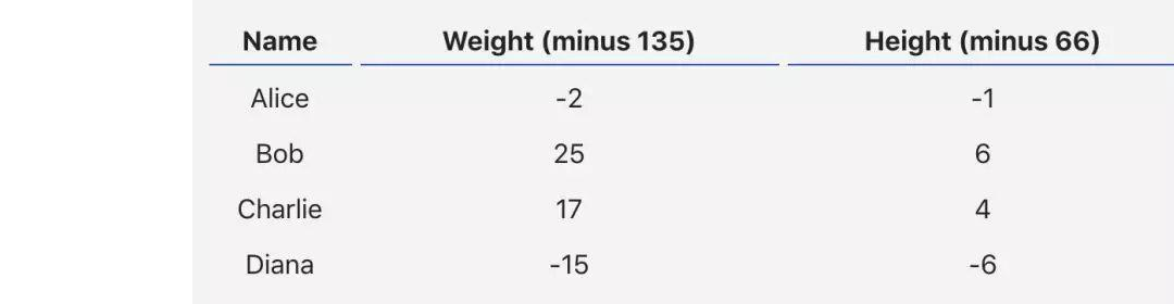
Assume there is a dataset containing the height and weight of 4 individuals;

Now our goal is to train a network to predict someone’s gender based on weight and height.

For simplicity, we will subtract a fixed value from each person’s height and weight, defining male gender as 1 and female gender as 0.

Before training the neural network, we need a standard to define how good it is so that we can improve it, which is called loss.

For example, we can define the loss using Mean Squared Error (MSE):

n is the number of samples, which is 4 in the above dataset;

y represents a person’s gender, where male is 1 and female is 0;

ytrue is the true values of the variable, and ypred is the predicted values of the variable.

As the name suggests, the Mean Squared Error is the average of the variances of all data, and we can define it as the loss function. The better the prediction, the lower the loss, and training the neural network is about minimizing the loss.

If the output of the above network is always 0, meaning predicting everyone as male, then the loss is:

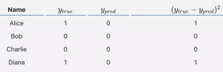
MSE= 1/4 (1+0+0+1)= 0.5

The code to calculate the loss function is as follows:

import numpy as np

def mse_loss(y_true, y_pred):

# y_true and y_pred are numpy arrays of the same length.

return ((y_true – y_pred) ** 2).mean()

y_true = np.array([1, 0, 0, 1])

y_pred = np.array([0, 0, 0, 0])

print(mse_loss(y_true, y_pred)) # 0.5 Reducing Neural Network Loss

This neural network is not good enough and needs to be continually optimized to minimize the loss. We know that changing the weights and biases of the network can affect the predicted values, but how should we do that?

For simplicity, we reduce the dataset to only contain Alice’s data. Thus, the loss function now only contains the variance of Alice:

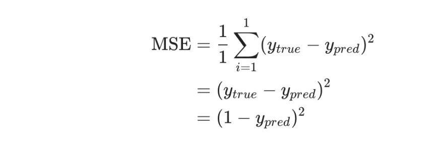
The predicted values are calculated from a series of network weights and biases:

Therefore, the loss function actually contains multiple weights and biases as a multivariable function:

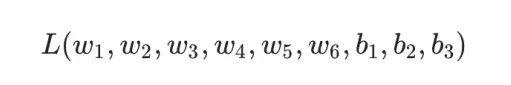
(Note! High energy ahead! You need to have some basic knowledge of multivariable function differentiation, such as partial derivatives and the chain rule.)

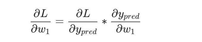
If we adjust w1, will the loss function increase or decrease? We need to know whether the partial derivative ∂L/∂w1 is positive or negative to answer this question.

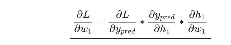
According to the chain rule:

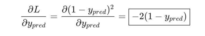
And L=(1-ypred)2, we can find the first partial derivative:

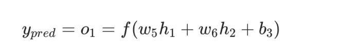
Next, we need to find the relationship between ypred and w1, and we already know the mathematical operation rules of neurons h1, h2, and o1:

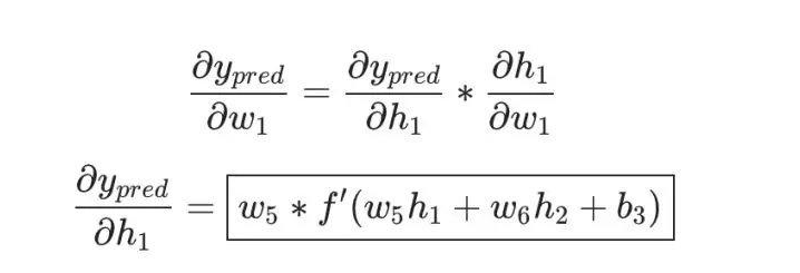
In fact, only the neuron h1 contains the weight w1, so we apply the chain rule again:

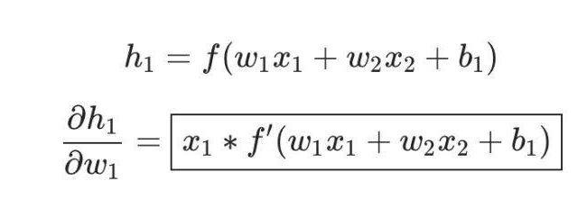
Then find ∂h1/∂w1

In our previous calculations, we encountered the derivative of the activation function sigmoid, denoted as f′(x), which is easy to calculate:

The overall chain rule formula:

This system for calculating partial derivatives backward is called backpropagation.

There are too many mathematical symbols above; let’s substitute actual values to calculate. h1, h2, and o1

h1=f(x1⋅w1+x2⋅w2+b1)=0.0474

h2=f(w3⋅x3+w4⋅x4+b2)=0.0474

o1=f(w5⋅h1+w6⋅h2+b3)=f(0.0474+0.0474+0)=f(0.0948)=0.524

The output of the neural network y=0.524 does not strongly indicate male (1) or female (0). The current prediction effect is still poor.

Let’s calculate the current network’s partial derivative ∂L/∂w1:

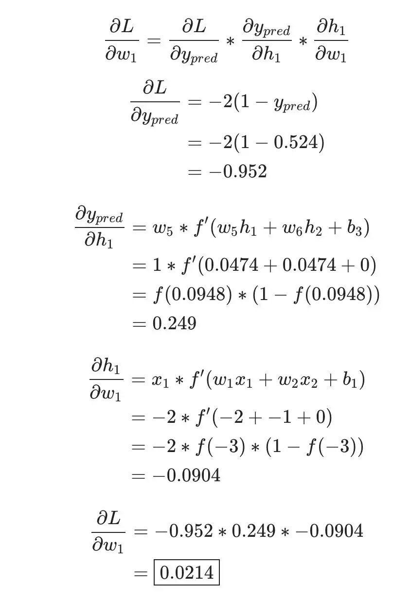
This result tells us: if we increase w1, the loss function L will increase slightly.

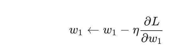
Next, we will use an optimization algorithm called Stochastic Gradient Descent (SGD) to train the network.

After the previous calculations, we have all the data needed to train the neural network. But how should we operate? SGD defines how to change weights and biases:

– data is a (n x 2) numpy array, n = # of samples in the dataset.

– all_y_trues is a numpy array with n elements.

Elements in all_y_trues correspond to those in data.

”’

learn_rate = 0.1

epochs = 1000 # number of times to loop through the entire dataset

for epoch in range(epochs):

for x, y_true in zip(data, all_y_trues):

# — Do a feedforward (we’ll need these values later)

sum_h1 = self.w1 * x[0] + self.w2 * x[1] + self.b1

h1 = sigmoid(sum_h1)

sum_h2 = self.w3 * x[0] + self.w4 * x[1] + self.b2

h2 = sigmoid(sum_h2)

sum_o1 = self.w5 * h1 + self.w6 * h2 + self.b3

o1 = sigmoid(sum_o1)

y_pred = o1

# — Calculate partial derivatives.

# — Naming: d_L_d_w1 represents “partial L / partial w1”

d_L_d_ypred = -2 * (y_true – y_pred)

# Neuron o1

d_ypred_d_w5 = h1 * deriv_sigmoid(sum_o1)

d_ypred_d_w6 = h2 * deriv_sigmoid(sum_o1)

d_ypred_d_b3 = deriv_sigmoid(sum_o1)

d_ypred_d_h1 = self.w5 * deriv_sigmoid(sum_o1)

d_ypred_d_h2 = self.w6 * deriv_sigmoid(sum_o1)

# Neuron h1

d_h1_d_w1 = x[0] * deriv_sigmoid(sum_h1)

d_h1_d_w2 = x[1] * deriv_sigmoid(sum_h1)

d_h1_d_b1 = deriv_sigmoid(sum_h1)

# Neuron h2

d_h2_d_w3 = x[0] * deriv_sigmoid(sum_h2)

d_h2_d_w4 = x[1] * deriv_sigmoid(sum_h2)

d_h2_d_b2 = deriv_sigmoid(sum_h2)

# — Update weights and biases

# Neuron h1

self.w1 -= learn_rate * d_L_d_ypred * d_ypred_d_h1 * d_h1_d_w1

self.w2 -= learn_rate * d_L_d_ypred * d_ypred_d_h1 * d_h1_d_w2

self.b1 -= learn_rate * d_L_d_ypred * d_ypred_d_h1 * d_h1_d_b1

# Neuron h2

self.w3 -= learn_rate * d_L_d_ypred * d_ypred_d_h2 * d_h2_d_w3

self.w4 -= learn_rate * d_L_d_ypred * d_ypred_d_h2 * d_h2_d_w4

self.b2 -= learn_rate * d_L_d_ypred * d_ypred_d_h2 * d_h2_d_b2

# Neuron o1

self.w5 -= learn_rate * d_L_d_ypred * d_ypred_d_w5

self.w6 -= learn_rate * d_L_d_ypred * d_ypred_d_w6

self.b3 -= learn_rate * d_L_d_ypred * d_ypred_d_b3

# — Calculate total loss at the end of each epoch

if epoch % 10 == 0:

y_preds = np.apply_along_axis(self.feedforward, 1, data)

loss = mse_loss(all_y_trues, y_preds)

print(“Epoch %d loss: %.3f” % (epoch, loss))

# Define dataset

data = np.array([

[-2, -1], # Alice

[25, 6], # Bob

[17, 4], # Charlie

[-15, -6], # Diana

])

all_y_trues = np.array([

1, # Alice

0, # Bob

0, # Charlie

1, # Diana

])

# Train our neural network!

network = OurNeuralNetwork()

network.train(data, all_y_trues)

As the learning process progresses, the loss function gradually decreases.

Now we can use it to predict each person’s gender:

# Make some predictions

emily = np.array([-7, -3]) # 128 pounds, 63 inches

frank = np.array([20, 2]) # 155 pounds, 68 inches

print(“Emily: %.3f” % network.feedforward(emily)) # 0.951 – F

print(“Frank: %.3f” % network.feedforward(frank)) # 0.039 – M