Editorial Team
WeChat Official Account
KeywordsFull Network SearchLatest Ranking
“Quantitative Investment”: Ranked First
“Quant”: Ranked First
“Machine Learning”: Ranked Fourth
We will continue to work hard
To become ahigh-qualityfinancial and technical public account
Translation by: mchoi
[Series 1]Neural Networks for Algorithm Trading Based on Multivariate Time Series(Click the title to read)
In this article, we will consider the regression prediction problem, design and test a new loss function for it, convert returns into some volatility, and check different metrics for these problems. The code can be found at the end.
Back to Return Prediction
First, let’s remember how to switch from the original time series to returns (or percentage changes/rates of change). If we want to predict these returns, we can convert all our dimensions to returns (open, high, low, close, volume) — they will be normalized data and a more appropriate approach — if we intend to better predict returns, we need to invest in the form of returns.
def data2change(data):
    change = pd.DataFrame(data).pct_change()
    change = change.replace([np.inf, -np.inf], np.nan)
    change = change.fillna(0.).values.tolist()
    return change
openp = data_original.ix[:, 'Open'].tolist()
highp = data_original.ix[:, 'High'].tolist()
lowp = data_original.ix[:, 'Low'].tolist()
closep = data_original.ix[:, 'Adj Close'].tolist()
volumep = data_original.ix[:, 'Volume'].tolist()
openp = data2change(openp)
highp = data2change(highp)
lowp = data2change(lowp)
closep = data2change(closep)
volumep = data2change(volumep)
Let’s define the neural network as usual and require it to minimize the loss function, and we will choose these functions as the new Mean Absolute Error (MAE). Particularly considering that in this case, if we predict a percentage, it will be easier to record, for example, an average error of 5%.
model = Sequential()
model.add(Convolution1D(input_shape = (WINDOW, EMB_SIZE),nb_filter=16,filter_length=4,border_mode='same'))
model.add(MaxPooling1D(2))
model.add(LeakyReLU())
model.add(Convolution1D(nb_filter=32,filter_length=4,border_mode='same'))
model.add(MaxPooling1D(2))
model.add(LeakyReLU())
model.add(Flatten())
model.add(Dense(16))
model.add(LeakyReLU())
model.add(Dense(1))
model.add(Activation('linear'))
opt = Nadam(lr=0.002)
reduce_lr = ReduceLROnPlateau(monitor='val_loss',factor=0.9, patience=25, min_lr=0.000001, verbose=1)
checkpointer = ModelCheckpoint(filepath="lolkekr.hdf5",verbose=1, save_best_only=True)
model.compile(optimizer=opt,loss='mae')
history = model.fit(X_train, Y_train,nb_epoch = 100,batch_size = 128,verbose=1,validation_data=(X_test, Y_test),callbacks=[reduce_lr, checkpointer],shuffle=True)
We obtained the following results:
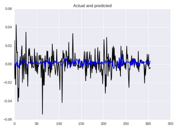
Neural Network Prediction Based on Mean Absolute Error
According to different metrics, we obtained MAE: 0.00013, MAE: 0.0082, MAPE: 144.4%
Let’s take a look at the errors closer to MAE:
Let’s remember what we intended to predict before — how much and in what direction it will change. Now I would like to ask you to read a small section about Bayesian methods:
Assume that the future return rate of a stock is very small, which is 0.01 (or 1%). We have a model for predicting future stock prices, and our gains and losses are directly related to the predictions. How should we measure the losses associated with model predictions and the subsequent predictions? A squared error loss is agnostic to the labels and is equally unfavorable for a prediction of 0.1 as it is for a prediction of 0.03. If you bet based on the model’s prediction, you will make a profit with a prediction of 0.03 and lose money with a prediction of -0.01, but our loss does not capture that. We need a better loss that considers the signs of the predictions and actual values.
We can now see that our current loss function MAE does not give us information about the direction of change! We will try to fix it.
Back to Custom Loss Function
Implementing it in Keras:
def stock_loss(y_true, y_pred):
    alpha = 100.
    loss = K.switch(K.less(y_true * y_pred, 0),alpha*y_pred**2-K.sign(y_true)*y_pred +K.abs(y_true),
    K.abs(y_true - y_pred))
    return K.mean(loss, axis=-1)
When implementing Keras’s “difficult” loss function, consider that operations like “if-else-less-equal” must be implemented through the appropriate backend, for example, the if-else statement block is implemented in my K.switch example.
We can see that if we correctly predict the direction (signal), that is the same as the mean absolute error (K.abs(y_true-y_pred)), but if not, we will penalize our loss for wrong signals (alpha * y_pred ** 2 – K.sign(y_true) * y_pred + K.abs(y_true)) parameter a is needed to control the amount of penalty. To apply this loss function to our model, we need to compile the model with it (parameter a).
Let’s check the results!
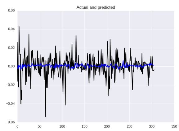
Neural Network Prediction Based on Mean Absolute Error
In terms of metrics, it is slightly better: MSE: 0.00013, MAE: 0.0081, and MAPE: 132%, but in our eyes this image still does not satisfy, the model cannot better predict the strength of volatility. This is a loss function issue, checking the results of previous articles, it is not very good, but also look at the predicted “size”.
As an exercise, try using the same approach — penalizing wrong signals (the original text is “penalyzing”, but I feel like it is the -ing form of the previous “penalize”) loss function — but using Mean Squared Error (MSE), as this loss function is more robust for regression problems.
Back to Volatility
First, we all agree that predicting when the market will “jump” is very important for this financial matter. Sometimes, the direction of the jump doesn’t matter — for example, in many young markets, like cryptocurrencies, a jump almost always means growth, or for example, a jump after a large but slow growth period is most likely to mean some decline, and these declines will give us a signal. In a sense, we are interested in predicting the “variability” of future prices.
This quantity of “variability” is called volatility (Wikipedia):
In finance, volatility (symbol σ) is a measure of the degree to which the trading price series varies over time, measured by the standard deviation of logarithmic returns.
We will use the standard deviation of price returns over the past N days and will attempt to predict the situation for the next day.
volatility = []
for i in range(WINDOW, len(data)):
window = highp[i-WINDOW:i]
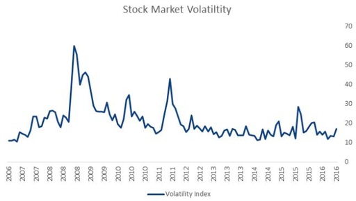
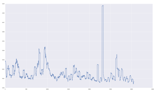
volatility.append(np.std(window))“Monthly Volatility” for GOOGL stocks is shown below:
Let’s check how we predict this quantity!
Volatility Prediction
for i in range(0, len(data_original), STEP):
    try:
        o = openp[i:i+WINDOW]
        h = highp[i:i+WINDOW]
        l = lowp[i:i+WINDOW]
        c = closep[i:i+WINDOW]
        v = volumep[i:i+WINDOW]
        volat = volatility[i:i+WINDOW]
        y_i = volatility[i+WINDOW+FORECAST]
        x_i = np.column_stack((volat, o, h, l, c, v))
We will adopt the same neural network architecture as above, change the loss function to MSE, and repeat the process of predicting volatility. The results are as follows:
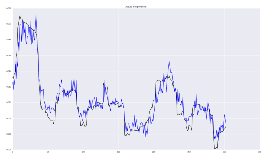
Overall, it doesn’t look bad! Of course, some jumps were predicted too late, but the ability to capture dependencies is good! In terms of metrics, MSE is 2.5426229985e-05, MAE is 0.0037, MAPE is 38%.
I also want to encourage everyone to try different loss functions, for example, from the one below. For example, let’s try using log MSE:
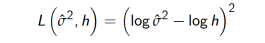
def mse_log(y_true, y_pred):
    y_pred = K.clip(y_pred, epsilon, 1.0 - epsilon)
    loss = K.square(K.log(y_true) - K.log(y_pred))
    return K.mean(loss, axis=-1)
model.compile(optimizer=opt, loss=mse_log)
Metrics are MSE 2.52380132336e-05, MAE 0.0037, and MAPE 37%. Not much, but already better! You can implement some other loss functions in the repository.
Code Showcase:
Followers
From1to10000+
We are making progress every day