Machine Heart Editorial Team
Training a fully connected network with 100 million parameters, a 44-core CPU makes the V100 bow down, and it turns out to be due to—hashing?
Accelerating training and inference of deep learning models has recently been a focus in the research field.Although the common view is that GPUs have a stronger computational advantage over CPUs.Recently, computer scientists from Rice University released new research results, proposing a deep learning framework that validates acceleration of deep learning without specialized hardware acceleration like GPUs on large-scale industrial recommendation datasets.
In the paper, the researchers pointed out that although existing studies show that optimizing models on the algorithm side does not exhibit the powerful performance improvements like those of the V100 GPU, their proposed SLIDE engine can achieve this. This model can significantly reduce computations during training and inference,being faster than algorithms highly optimized for TensorFlow on a GPU.
For instance, when testing SLIDE on industrial-scale recommendation datasets,the training time on Tesla V100 GPU is 3.5 times that of Intel Xeon E5-2699A 2.4GHz.Under the same CPU hardware conditions,SLIDE is 10 times faster than TensorFlow.
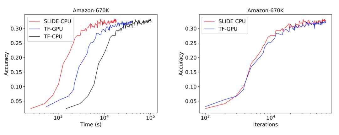
We can first look at an experimental graph, where the training time for a large neural network with over 100 million parameters on a complex classification dataset like Amazon-670K is surprisingly fastest with SLIDE + CPU, much slower than TensorFlow + Tesla V100.Moreover, from the number of iterations, the two are equivalent, indicating that the model’s convergence behavior is the same.
For the reproduction of the paper and results, the researchers have provided the corresponding code.
Significant Reduction in Computational Complexity, Locality Sensitive Hashing Works Wonders
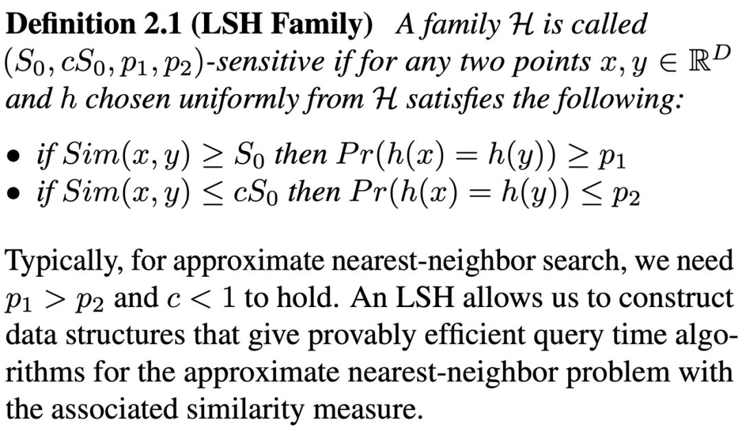
How is such a miraculous acceleration achieved?Specifically, the researchers adopted the Locality Sensitive Hashing (LSH) algorithm and used adaptive dropout in the neural network.Locality Sensitive Hashing is a class of hash algorithms that has a higher collision probability when input data is similar, while the probability of collision is low for dissimilar algorithms.A widely used nearest neighbor approximation search algorithm employs the theory of locality sensitive hashing.
How SLIDE Constructs Locality Sensitive Hashing
In a 1998 study by Indyk and Motwani, it was shown that for a given similarity computation, a class of LSH functions is sufficient to effectively solve nearest neighbor search in sub-linear time.
Algorithm:LSH algorithm uses two parameters (K, L), the researchers constructed L independent hash lists.Each hash table has an original hash function H, which is formed by concatenating K random independent hash functions from the set F.Given a query, one bucket is collected from each hash list, returning a set of L buckets.
Intuitively, the original hash function makes the buckets sparse and reduces the number of false positives because only valid nearest neighbors can match all K hash values for the query.The bucket set of L reduces the number of false negatives by increasing the potential number of buckets that can hold the nearest neighbors.The candidate generation algorithm works in two phases:
1. Preprocessing phase, by storing all x elements, constructing L hash lists at the data level.Only pointers to vectors in the hash list are stored because storing entire data vectors would be very inefficient.
2. Query phase:Given a query Q,search for its nearest neighbors, reporting from the set of all buckets collected from L hash lists.Note that there is no need to scan all elements, only probing different buckets of L, where each hash list has one bucket.
After generating potential candidate algorithms, the nearest neighbors are calculated by comparing the distance between each item in the candidate set and the query.
Using Locality Sensitive Hashing for Sampling and Estimation
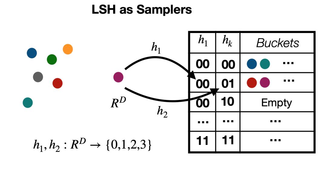
Although locality sensitive hashing has been shown to allow for rapid extraction under sub-linear conditions, it is very slow for exact searches because it requires a large number of hash tables.Research has shown that efficient sampling as shown in Figure 1 can alleviate the computational load of searches to some extent, allowing sufficient adaptive sampling by looking at only some hash buckets.
Figure 1:Illustration of Locality Sensitive Hashing.For an input, hash codes can be extracted from the corresponding hash buckets.
Recent research on maximum inner product search (MIPS) has also demonstrated this, where asymmetric locality sensitive hashing can make sampling large inner products feasible.Given a set of vectors C and a query vector Q.Using the (K, L)-parameterized LSH algorithm and MIPS hash, a candidate set S can be obtained.Here, only a linear cost is needed to preprocess hashing C, while for Q, only a small amount of hash lookup work is required.
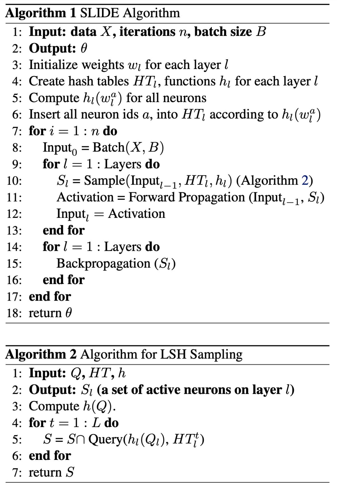
Algorithms in SLIDE, including framework (Algorithm 1) and hash sampling (Algorithm 2).
Building the SLIDE System
Figure 2:SLIDE system architecture.
In the SLIDE architecture, the core module is the network.This neural network is composed of several single-layer modules.Each layer’s module consists of neurons and some hash tables—converting neuron IDs into hashes.
For each neuron, it has multiple arrays of batch size length:1) A binary array indicating whether each input activates this neuron;2) Activation of each input;3) Cumulative gradients for each input in the batch;4) Connection weights between this layer and the previous layer;5) The number of neurons in the previous layer, represented by the last array.
Each layer object contains a list of neurons and a set of LSH sampling hash lists.Each hash list contains the IDs of neurons hashed into buckets.During the network initialization process, the network’s weight values are randomly initialized.Then, L hash lists are used to initialize K * L LSH functions for each layer.
Sparse Forward Propagation Using Hash Table Sampling
In the forward propagation phase, given a single training instance, the researchers compute the activations of the network up to the last layer and produce output.In SLIDE, they do not compute all activations of each layer but input each layer’s input xl into the hash function, obtaining hl(xl), using the hash code as a query to get the IDs of activated (sampled) neurons from the corresponding matching buckets.
Sparse Backward Propagation / Gradient Update
The backward propagation step follows immediately after forward propagation.After calculating the neural network’s output, the researchers compare the output with the labels and backpropagate the error layer by layer to compute gradients and update weights.Here they use the classic backpropagation method.
Updating Hash Lists After Weight Update
After updating weight values, the positions of neurons in the hash lists need to be adjusted accordingly.Updating neurons typically involves deleting from old hash buckets and then adding new content from new hash buckets, which can be very time-consuming.Section 4.2 will discuss several design techniques to optimize the expensive overhead caused by updating hash lists.
OpenMP Cross-Batch Processing Parallelization
For any given training instance, the feedforward and backward propagation operations are sequential because they need to be executed layer by layer.SLIDE uses common batch gradient descent methods and the Adam optimizer, with batch sizes typically around a few hundred.Each data instance’s run in the batch is in a separate thread, and its gradient is computed in parallel.
The extreme sparsity and randomness of gradient updates allow us to accumulate gradients on different training data through asynchronous parallel processing without causing significant overlapping updates.SLIDE extensively uses the theory of HOGWILD (Recht et al., 2011), showing that a small amount of overlap is manageable.
Truth → CPU Faster than GPU
The researchers attached a series of experimental results at the end of the paper, including comparisons of TensorFlow models using Tesla V100 GPU, TensorFlow models using two Intel Xeon E5-2699A CPUs (single 22-core, total 44 cores), and performance comparisons between SLIDE adaptive sampling and sampled Softmax.We can find that SLIDE’s training speed on CPU is surprisingly efficient.
First, for the test model, the researchers used a super fully connected model with 100 million parameters, and the datasets are large industrial classification datasets like Delicious200K and Amazon-670K.These two datasets have over 780,000 and over 130,000 feature dimensions, and over 200,000 and over 670,000 categories, which looks terrifying.Due to the high feature dimensions and classification categories, even with few hidden layer units, the overall parameter count will surge.
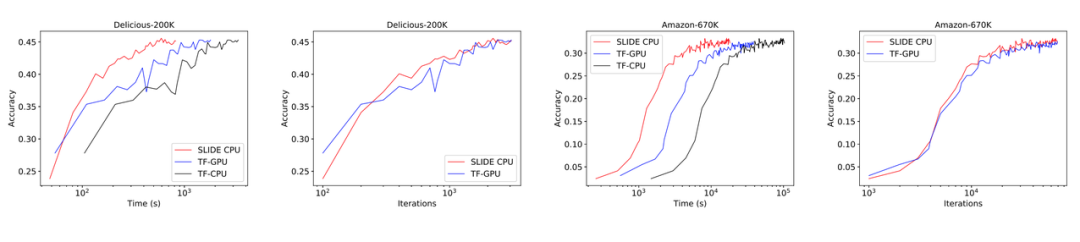
The following figure shows the main results of the paper, where SLIDE on CPU is faster than V100 (using TensorFlow framework), and consistently outperforms the CPU-based TF model.
Figure 5:Comparison of effects between SLIDE (red line), TF-GPU (blue line), and TF-CPU (black line).
On the Delicious200K dataset, SLIDE is 1.8 times faster than TF-GPU.On the more computationally demanding Amazon-670K, the convergence time of TF-GPU is 2.7 times that of SLIDE (2 hours vs. 5.5 hours).In terms of iterations, the convergence behaviors of both are equivalent, except that SLIDE is faster in each iteration.
Moreover, in Figure 5, the final convergence effects are similar, indicating that under the SLIDE framework, the model’s performance is not compromised.
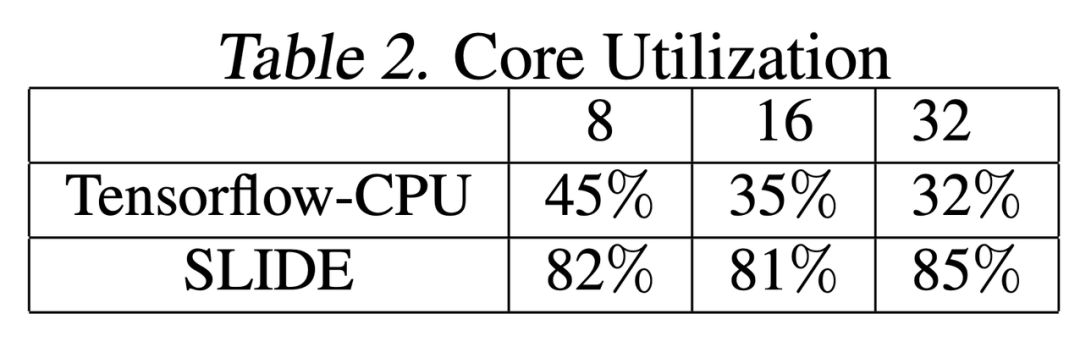
Table 2 shows the CPU core usage, testing the framework under 8, 16, and 32 threads.We can see that for TF-CPU, its utilization is very low (<50%), and as the number of threads increases, the utilization further decreases.For SLIDE, the utilization of computational cores is very stable, around 80%.
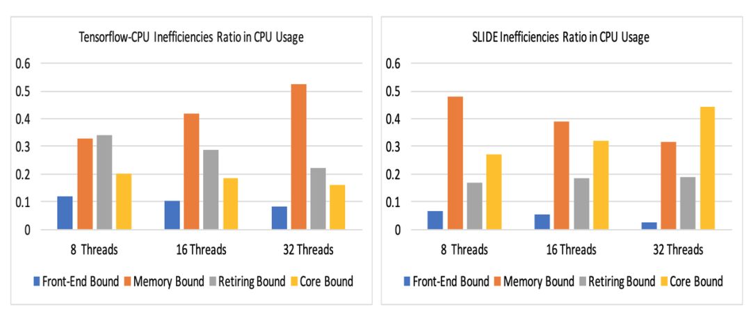
Figure 6 shows the distribution of ineffective CPU utilization between TF-CPU and SLIDE.SLIDE’s utilization of computational cores is much higher than that of TF-CPU.
Figure 6:Ineffective CPU utilization:Memory-bound low utilization (orange) is most significant for both algorithms.TF-CPU’s memory-bound low utilization increases with the number of cores, while SLIDE decreases.
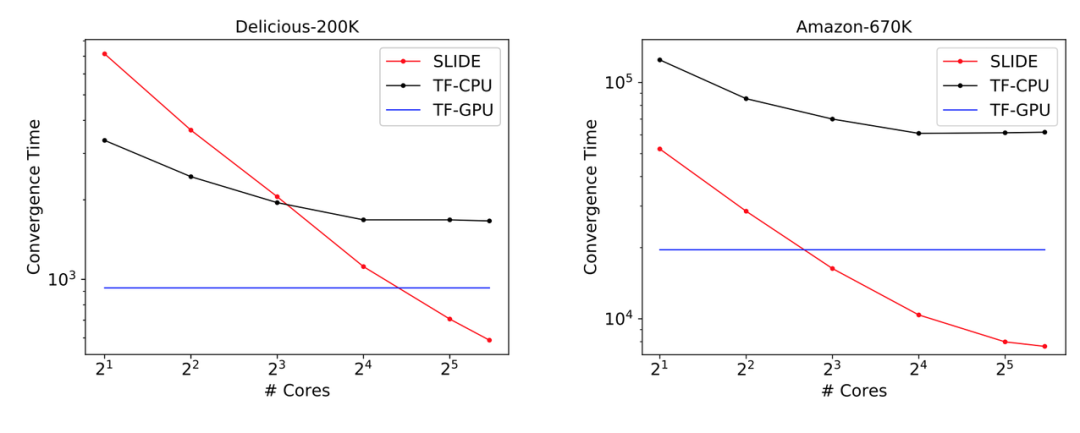
Due to its efficient use of CPU computational resources, SLIDE can significantly reduce convergence time as the number of CPU cores increases.
Figure 9:Scalability tests between TF-CPU and SLIDE, showing that SLIDE is significantly stronger.
SLIDE is now open-source.In the open-source project, the authors provide datasets and corresponding code for testing.
First, users need to install CNPY and enable Transparent Huge Pages, as SLIDE requires about 900 pages, each 2MB, and 10 pages of 1GB.
The process to run the code is as follows:
make ./runme Config_amz.csv
It is important to note that the Makefile needs to modify the path based on CNPY, and modifications are required in Config_amz.csv for trainData, testData, logFile, etc.
As for the training data, it comes from Amazon-670K, and the download link is as follows:
https://drive.google.com/open?id=0B3lPMIHmG6vGdUJwRzltS1dvUVk
In the industrial field, model structures are not necessarily very complex, as simple models like Naive Bayes and fully connected networks often receive more preference.However, real models are usually very large, and configuring high-performance GPUs to train models is very uneconomical.Even though this paper only validates fully connected networks, it at least demonstrates that high-performance CPUs can indeed meet the training needs of large models, significantly reducing hardware costs.
Machine Heart and WeBank jointly launched an online open course titled “Introduction and Application Practice of Federated Learning FATE,” lasting 4 weeks, with 6 sessions, featuring keynote speeches + project practice + online Q&A, starting from zero in federated learning. The first lesson of the series will begin on March 5. Add the Machine Heart assistant to join the learning plan for free.