 The learning of artificial neural networks mainly refers to the use of learning algorithms to adjust the connection weights between neurons, so that the network output better matches reality. Learning algorithms are divided into supervised learning and unsupervised learning.
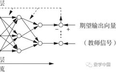
Supervised learning, also known as teacher-based learning, is a learning method where a set of training data is fed into the network. Based on the difference between the actual output of the network and the expected output, the connection weights are adjusted. The expected output, also known as the teacher signal, serves as the evaluation standard for learning.
The results obtained from supervised learning cannot guarantee an optimal solution; it requires a large training sample, converges slowly, and is sensitive to the order of sample presentation.
1. BP Algorithm
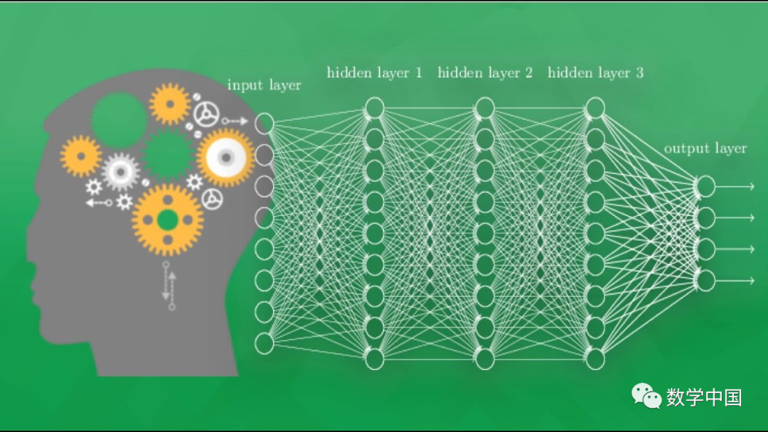
The BP algorithm is short for the error backpropagation training algorithm. It systematically solves the problem of learning connection weights of hidden units in multi-layer networks and has strong nonlinear mapping capabilities. A three-layer BP neural network algorithm can approximate any nonlinear function and is currently one of the most widely used networks.
The structure of a multi-layer feedforward network based on the BP algorithm is shown in Figure 1.
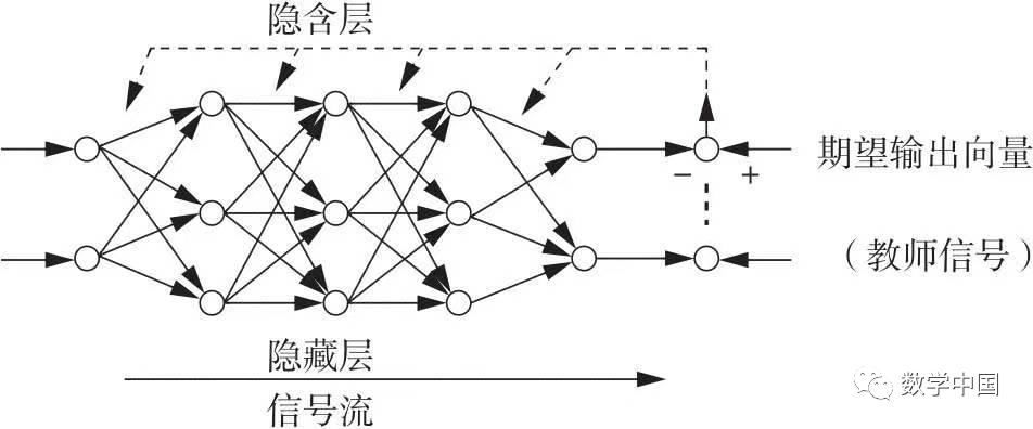
Figure 1: Structure of a Multi-Layer Feedforward Network Based on the BP Algorithm
This network has not only input layer nodes and output layer nodes, but also one or more layers of hidden nodes. BP networks are generally three-layered, while four layers or more are used less frequently. For multi-layer feedforward networks, determining the number of hidden layer nodes is key to success. If the number is too small, the network will have too little information to solve the problem; if the number is too large, it will not only increase training time but also potentially lead to the so-called “overfitting” problem, where the testing error increases and generalization capability decreases. Therefore, it is crucial to choose the number of hidden layer nodes reasonably. The selection of the number of hidden layers and their nodes is complex, but the general principle is to choose fewer hidden layer nodes to keep the network structure as simple as possible while correctly reflecting the input-output relationship.
For input information, it first propagates forward to the hidden layer nodes. After passing through each unit’s activation function (also known as the action function or transfer function), the output information of the hidden nodes is propagated to the output nodes, finally giving the output result. The learning process of the network consists of forward and backward propagation. In the forward propagation process, the state of each layer of neurons only affects the next layer of neurons. If the output layer cannot obtain the expected output, which means there is an error between the actual output value and the expected output value, the process shifts to backward propagation. The error signal is returned along the original connection path, adjusting the weights of each layer of neurons, and propagating back to the input layer for computation, followed by the forward propagation process. The repeated use of these two processes minimizes the error signal. In fact, when the error meets the desired requirement, the learning process of the network ends.
The BP algorithm is a teacher-guided learning method suitable for multi-layer neural networks, based on the gradient descent method. Theoretically, a BP network with one hidden layer can approximate any continuous nonlinear function to any desired accuracy.
Assuming an arbitrary network with L layers and n nodes, each layer unit only accepts input information from the previous layer and outputs to the next layer units. Each node (sometimes called a unit) has a Sigmoid-type characteristic (which is continuous and differentiable, unlike the linear threshold function in perceptrons, which is discontinuous). For simplicity, assume the network has only one output y. Given N samples (xk, yk) (k=1,2,…,N), the output of any node i is Oi. For a given input xk, the network output is yk, and the output of node i is Oik. Now we study the j-th unit of the l-th layer when inputting the k-th sample, where the input to node j is:
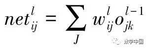
, the output is: 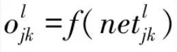 , where
  represents the output of node j in the (l-1) layer when inputting the k-th sample. The error function used is:
 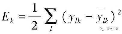 , where
  is the actual output of unit j. The total error is:
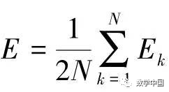 .Definition:
 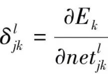 , thus:
.
Discussing in two cases:
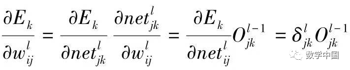
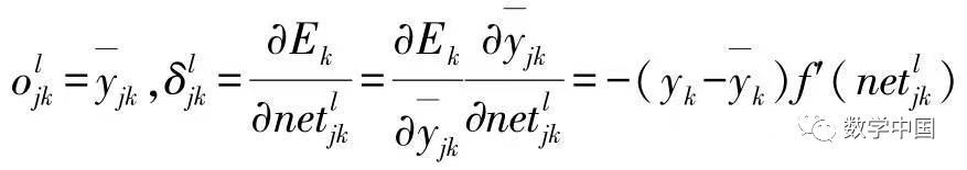
If node j is an output unit, then
If node j is not an output unit, then
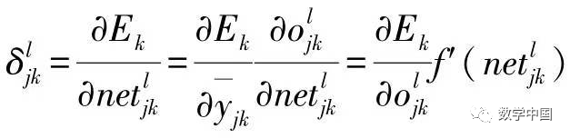 , where
  is the input sent to the next layer (l+1), and calculating
 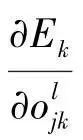 needs to be computed from layer (l+1). In the m-th unit of layer (l+1):
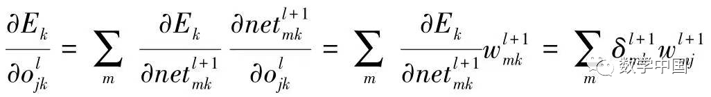
Substituting and simplifying gives: 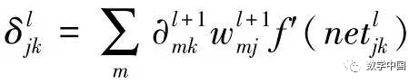 Summarizing the above results, we have:

2. Delta Learning Rule
The Delta learning rule is a simple teacher-based learning algorithm that adjusts the connection weights based on the difference between the actual output of the neuron and the expected output. The mathematical expression is
wij(t+1) = wij(t) + α(di – yi)xj(t)
where wij represents the connection weight from neuron j to neuron i; di is the expected output of neuron i; yi is the actual output of neuron i; xj is the state of neuron j. If neuron j is in an activated state, then xj = 1; if neuron j is in an inhibited state, depending on the activation function, xj = 0 or xj = -1; α is a constant that represents the learning rate. Assuming xi = 1, if di is greater than yi, then wij will increase; if di is less than yi, then wij will decrease.
In simple terms, the Delta learning rule states that if the actual output of the neuron is greater than the expected output, decrease all positive input connection weights and increase all negative input connection weights. Conversely, if the actual output of the neuron is less than the expected output, increase all positive input connection weights and decrease all negative input connection weights. The magnitude of this increase or decrease is calculated based on the above expression.
3. Introduction to Unsupervised Learning
Unsupervised learning, also known as teacherless learning, extracts the statistical features contained in the sample set and stores them in the network in the form of connection weights between neurons. In unsupervised learning, no teacher signal is provided to the neural network; the neural network adjusts the connection weight coefficients and thresholds based solely on its input. At this point, the evaluation standard for the network’s learning is implicit within itself. This learning method mainly accomplishes clustering operations.
One representative algorithm in unsupervised learning is the Hebb algorithm. The core idea of the Hebb algorithm is that when two neurons are simultaneously in an excited state, the connection weight between them will be strengthened; otherwise, it will be weakened. The mathematical expression of the Hebb algorithm is wij(t+1) = wij(t) + αyj(t)yi(t) where wij represents the connection weight from neuron j to neuron i, and yi and yj are the outputs of the two neurons; α is a constant that represents the learning rate. If yi and yj are both activated, meaning they are both positive, then wij will increase; if yi is activated and yj is in an inhibited state, meaning yi is positive and yj is negative, then wij will decrease.