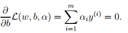
Source : Turing Artificial Intelligence
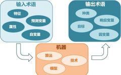
According to the different types of data, modeling a problem can be done in various ways. In the field of machine learning or artificial intelligence, the learning method of the algorithm is usually the first consideration. There are several main learning methods in machine learning. Classifying algorithms by learning methods is a good idea, as it allows people to choose the most suitable algorithm based on input data to achieve the best results.
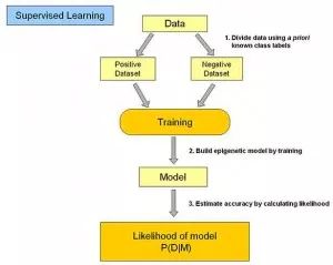
1. Supervised Learning:
In supervised learning, the input data is referred to as “training data,” and each set of training data has a clear label or result, such as “spam” or “not spam” in anti-spam systems, or “1,” “2,” “3,” “4,” etc., in handwritten digit recognition. When building a predictive model, supervised learning establishes a learning process that compares the predicted results with the actual results of the “training data,” continuously adjusting the predictive model until the model’s predictions reach an expected accuracy.Common applications of supervised learning include classification and regression problems.Common algorithms include Logistic Regression and Back Propagation Neural Network.
2. Unsupervised Learning:
In unsupervised learning, the data is not specifically labeled, and the learning model is designed to infer some intrinsic structure of the data.Common application scenarios include learning association rules and clustering.Common algorithms include Apriori and k-Means.
3. Semi-supervised Learning:
In this learning method, some input data is labeled while some is not. This learning model can be used for prediction, but the model first needs to learn the intrinsic structure of the data to organize it appropriately for predictions. Application scenarios include classification and regression, and algorithms include extensions of common supervised learning algorithms that first attempt to model the unlabeled data and then predict the labeled data based on that. For example, Graph Inference algorithms or Laplacian SVM.
4. Reinforcement Learning:
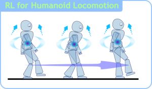
In this learning mode, input data serves as feedback to the model. Unlike supervised models, where the input data merely serves as a way to check the correctness of the model, in reinforcement learning, the input data directly feeds back into the model, which must make immediate adjustments. Common application scenarios include dynamic systems and robot control.Common algorithms include Q-Learning and Temporal Difference Learning.
In the context of enterprise data applications, the most commonly used models are probably supervised and unsupervised learning. In fields like image recognition, where there are large amounts of unlabeled data and a small amount of labeled data, semi-supervised learning is currently a hot topic. Reinforcement learning is more commonly applied in robot control and other areas requiring system control.
5. Algorithm Similarity
Based on the functional and formal similarities of algorithms, we can classify them, such as tree-based algorithms, neural network-based algorithms, etc. Of course, the scope of machine learning is very vast, and some algorithms are hard to classify into a single category. For some classifications, algorithms within the same category can target different types of problems.Here, we try to classify commonly used algorithms in the most understandable way.
6. Regression Algorithms:
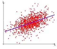
Regression algorithms attempt to explore the relationships between variables by measuring errors.Regression algorithms are powerful tools in statistical machine learning.In the field of machine learning, when people refer to regression, it may sometimes refer to a type of problem or sometimes to a type of algorithm, which can often confuse beginners. Common regression algorithms include: Ordinary Least Squares, Logistic Regression, Stepwise Regression, Multivariate Adaptive Regression Splines, and Locally Estimated Scatterplot Smoothing.
7. Instance-based Algorithms:
Instance-based algorithms are often used to build models for decision problems. Such models often first select a batch of sample data, then compare new data with the sample data based on certain similarities. This way of finding the best match is why instance-based algorithms are often referred to as “winner-takes-all” learning or “memory-based learning.” Common algorithms include k-Nearest Neighbor (KNN), Learning Vector Quantization (LVQ), and Self-Organizing Map (SOM).
8. Regularization Methods:
Regularization methods are extensions of other algorithms (usually regression algorithms), adjusting algorithms based on their complexity.Regularization methods generally reward simple models and penalize complex algorithms.Common algorithms include Ridge Regression, Least Absolute Shrinkage and Selection Operator (LASSO), and Elastic Net.
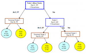
9. Decision Tree Learning:
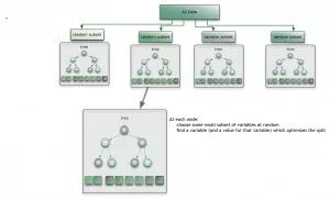
Decision tree algorithms establish decision models based on the attributes of the data, and decision tree models are often used to solve classification and regression problems. Common algorithms include Classification And Regression Tree (CART), ID3 (Iterative Dichotomiser 3), C4.5, Chi-squared Automatic Interaction Detection (CHAID), Decision Stump, Random Forest, Multivariate Adaptive Regression Splines (MARS), and Gradient Boosting Machine (GBM).
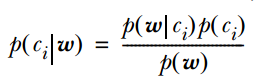
10. Bayesian Methods:
Bayesian method algorithms are a class of algorithms based on Bayes’ theorem, primarily used for solving classification and regression problems. Common algorithms include Naive Bayes, Averaged One-Dependence Estimators (AODE), and Bayesian Belief Network (BBN).
11. Kernel-based Algorithms:
Kernel-based algorithms are best exemplified by Support Vector Machines (SVM). These algorithms map input data into a higher-dimensional vector space, where some classification or regression problems can be solved more easily. Common kernel-based algorithms include Support Vector Machine (SVM), Radial Basis Function (RBF), and Linear Discriminant Analysis (LDA).
12. Clustering Algorithms:
Clustering, like regression, sometimes refers to a type of problem and sometimes to a type of algorithm. Clustering algorithms typically merge input data based on center points or hierarchical methods.All clustering algorithms attempt to find the intrinsic structure of the data to classify it based on the maximum commonalities.Common clustering algorithms include k-Means and Expectation Maximization (EM).
13. Association Rule Learning:
Association rule learning seeks to find rules that best explain the relationships between data variables, uncovering useful association rules in large multi-dimensional data sets. Common algorithms include Apriori and Eclat.
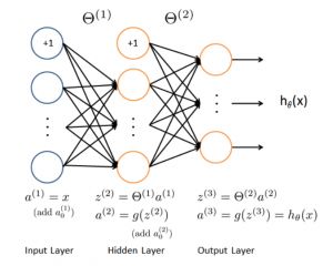
14. Artificial Neural Networks:
Artificial neural network algorithms simulate biological neural networks and are a class of pattern matching algorithms. They are typically used to solve classification and regression problems. Artificial neural networks are a vast branch of machine learning, with hundreds of different algorithms (including deep learning, which is one category we will discuss separately). Important artificial neural network algorithms include Perceptron Neural Network, Back Propagation, Hopfield Network, Self-Organizing Map (SOM), and Learning Vector Quantization (LVQ).
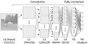
15. Deep Learning:
Deep learning algorithms are developments of artificial neural networks. They have gained significant attention recently, especially since Baidu has begun to focus on deep learning, which has attracted a lot of attention domestically. With the increasing affordability of computational power, deep learning aims to establish much larger and more complex neural networks. Many deep learning algorithms are semi-supervised learning algorithms used to handle large datasets with a small amount of unlabeled data. Common deep learning algorithms include Restricted Boltzmann Machines (RBM), Deep Belief Networks (DBN), Convolutional Networks, and Stacked Auto-encoders.
16. Dimensionality Reduction Algorithms:
Like clustering algorithms, dimensionality reduction algorithms attempt to analyze the intrinsic structure of the data. However, dimensionality reduction algorithms use an unsupervised learning approach to summarize or explain data using less information.This type of algorithm can be used for visualizing high-dimensional data or simplifying data for supervised learning.
Common algorithms include Principal Component Analysis (PCA), Partial Least Squares Regression (PLS), Sammon Mapping, Multi-Dimensional Scaling (MDS), and Projection Pursuit.
17. Ensemble Algorithms:
Ensemble algorithms train several relatively weak learning models independently on the same sample and then combine the results for overall predictions. The main challenge of ensemble algorithms is determining which independent weak learning models to include and how to integrate the learning results.
This is a very powerful and popular class of algorithms. Common algorithms include Boosting, Bootstrapped Aggregation (Bagging), AdaBoost, Stacked Generalization (Blending), Gradient Boosting Machine (GBM), and Random Forest.
Common Advantages and Disadvantages of Machine Learning Algorithms:
1. If the given feature vector lengths may differ, they need to be normalized to a common length vector (taking text classification as an example), for instance, if it is a sentence of words, then the length is the total vocabulary size, with corresponding positions being the occurrence counts of those words.
2. The computation formula is as follows:
One of the conditional probabilities can be expanded using the naive Bayes condition independence. It is important to note that  is calculated as follows, and based on the premise of naive Bayes, we know that
 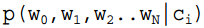 =
= , thus generally there are two methods, one is to find the total occurrences of wj in the samples where the category is ci, and then divide by the total of that sample; the second method is to find the total occurrences of wj in the samples where the category is ci, and then divide by the total occurrences of all features in that sample.
3. If
, thus generally there are two methods, one is to find the total occurrences of wj in the samples where the category is ci, and then divide by the total of that sample; the second method is to find the total occurrences of wj in the samples where the category is ci, and then divide by the total occurrences of all features in that sample.
3. If  contains a zero, then the product of the joint probabilities may also be zero, meaning that the numerator in the formula from 2 becomes zero. To avoid this situation, generally, this item is initialized to 1, and of course, to ensure probability equality, the denominator should be initialized to 2 (here because there are 2 categories, so we add 2; if there are k categories, we need to add k, a term called Laplace smoothing, where the denominator is increased by k to satisfy the total probability formula).
Advantages of Naive Bayes: It performs well on small-scale data, is suitable for multi-class tasks, and is apt for incremental training.
Disadvantages: It is very sensitive to the expression form of input data.
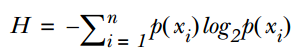
Decision Trees: One important aspect of decision trees is selecting an attribute for branching, so attention should be paid to the calculation formula of information gain and a deep understanding of it.
The calculation formula for information entropy is as follows:
where n represents n categories (for example, if it is a 2-class problem, then n=2). Calculate the probabilities p1 and p2 of these 2 categories in the total samples, and thus we can calculate the information entropy before selecting the attribute for branching.
Now, selecting an attribute xi for branching, the branching rule is: if xi=vx, the sample goes to one branch of the tree; if not equal, it goes to another branch. It is clear that the samples in the branch are likely to include 2 categories; calculate the entropy H1 and H2 of these 2 branches, and calculate the total information entropy after branching H’=p1*H1+p2*H2. Then the information gain ΔH=H-H’. By using information gain as a principle, test all attributes and select the one that yields the maximum gain as the branching attribute for this time.
Advantages of Decision Trees: They have simple computation, strong interpretability, are relatively suitable for handling samples with missing attribute values, and can handle irrelevant features;
Disadvantages: They are prone to overfitting (subsequently, Random Forest was introduced to reduce overfitting).
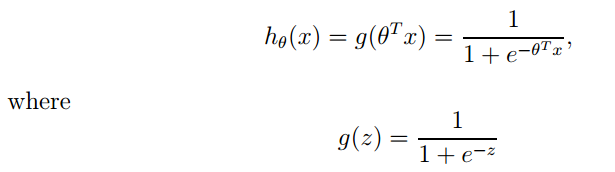
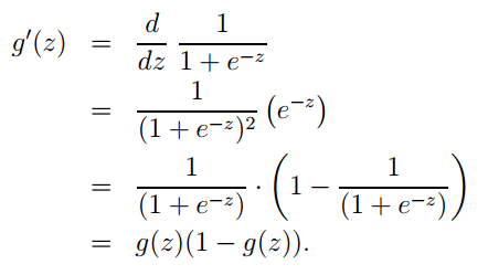
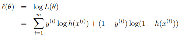
Logistic Regression: Logistic regression is used for classification and is a linear classifier. Points to note include:
1. The logistic function expression is:
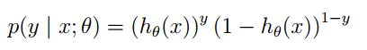
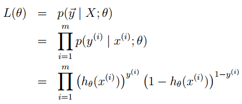
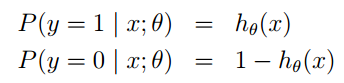
2. The logistic regression method primarily learns using maximum likelihood estimation, so the posterior probability of a single sample is:
For the posterior probability of the entire sample:
Through logs, it can be further simplified to:
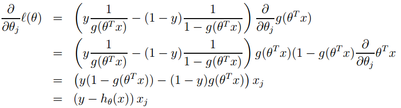
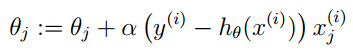
3. Its loss function is -l(θ), so we need to minimize the loss function, which can be achieved using the gradient descent method. The formula for the gradient descent method is:
Advantages of Logistic Regression:
2. Very fast computation during classification, low storage resource usage.
1. Prone to underfitting, generally low accuracy.
2. Can only handle binary classification problems (softmax derived from this can be used for multi-class), and must be linearly separable.
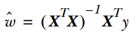
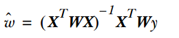
Linear regression is genuinely used for regression, unlike logistic regression which is used for classification. Its basic idea is to optimize the error function in the form of least squares using the gradient descent method. Of course, it can also directly solve the parameter using the normal equation, resulting in:
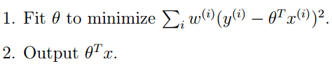
In LWLR (Locally Weighted Linear Regression), the parameter calculation expression is:
Because at this point, the optimization is:
It can be seen that LWLR differs from LR in that LWLR is a non-parametric model since each regression calculation requires traversing the training samples at least once.
Advantages of Linear Regression: Simple implementation, simple computation;
Disadvantages: Cannot fit non-linear data;
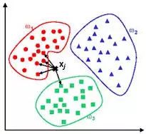
KNN Algorithm:KNN, or the k-Nearest Neighbors algorithm, primarily follows these steps:
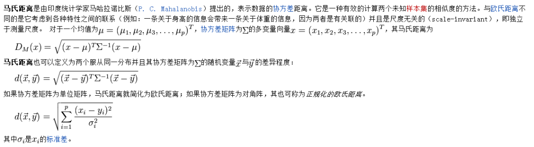
1. Calculate the distance between each sample point in the training set and the test sample (common distance metrics include Euclidean distance, Mahalanobis distance, etc.);
2. Sort all the distance values obtained above;
3. Select the top k samples with the smallest distances;
4. Vote based on the labels of these k samples to determine the final classification category;
How to choose the best K value depends on the data. Generally, a larger K value can reduce the impact of noise. However, it can make the boundaries between categories more ambiguous. A good K value can be obtained through various heuristic techniques, such as cross-validation.Additionally, the presence of noise and irrelevant feature vectors can reduce the accuracy of the K-Nearest Neighbors algorithm.
The nearest neighbor algorithm has strong consistency results. As the data approaches infinity, the algorithm guarantees that the error rate will not exceed twice the error rate of the Bayesian algorithm. For some good K values, K-Nearest Neighbors guarantees that the error rate will not exceed the Bayesian theoretical error rate.
Note: Mahalanobis distance must first provide the statistical properties of the sample set, such as mean vector, covariance matrix, etc. The introduction to Mahalanobis distance is as follows:
KNN Algorithm Advantages:
1. Simple idea, mature theory, can be used for both classification and regression;
2. Can be used for non-linear classification;
3. Training time complexity is O(n);
4. High accuracy, no assumptions about data, insensitive to outliers;
1. High computational load;
2. Sample imbalance issue (i.e., some categories have many samples while others have few);
3. Requires a large amount of memory;
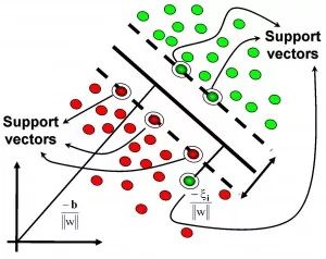
Learn how to use libsvm and some parameter tuning experiences, and clarify some thoughts on the SVM algorithm:
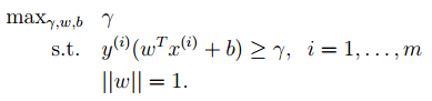
1. The optimal classification surface in SVM maximizes the geometric margin for all samples (why choose the maximum margin classifier? Please explain from a mathematical perspective; this has been asked during interviews for deep learning positions at NetEase. The answer is that there is a relationship between the geometric margin and the number of misclassifications of samples:
contains a zero, then the product of the joint probabilities may also be zero, meaning that the numerator in the formula from 2 becomes zero. To avoid this situation, generally, this item is initialized to 1, and of course, to ensure probability equality, the denominator should be initialized to 2 (here because there are 2 categories, so we add 2; if there are k categories, we need to add k, a term called Laplace smoothing, where the denominator is increased by k to satisfy the total probability formula).
Advantages of Naive Bayes: It performs well on small-scale data, is suitable for multi-class tasks, and is apt for incremental training.
Disadvantages: It is very sensitive to the expression form of input data.
Decision Trees: One important aspect of decision trees is selecting an attribute for branching, so attention should be paid to the calculation formula of information gain and a deep understanding of it.
The calculation formula for information entropy is as follows:
where n represents n categories (for example, if it is a 2-class problem, then n=2). Calculate the probabilities p1 and p2 of these 2 categories in the total samples, and thus we can calculate the information entropy before selecting the attribute for branching.
Now, selecting an attribute xi for branching, the branching rule is: if xi=vx, the sample goes to one branch of the tree; if not equal, it goes to another branch. It is clear that the samples in the branch are likely to include 2 categories; calculate the entropy H1 and H2 of these 2 branches, and calculate the total information entropy after branching H’=p1*H1+p2*H2. Then the information gain ΔH=H-H’. By using information gain as a principle, test all attributes and select the one that yields the maximum gain as the branching attribute for this time.
Advantages of Decision Trees: They have simple computation, strong interpretability, are relatively suitable for handling samples with missing attribute values, and can handle irrelevant features;
Disadvantages: They are prone to overfitting (subsequently, Random Forest was introduced to reduce overfitting).
Logistic Regression: Logistic regression is used for classification and is a linear classifier. Points to note include:
1. The logistic function expression is:
2. The logistic regression method primarily learns using maximum likelihood estimation, so the posterior probability of a single sample is:
For the posterior probability of the entire sample:
Through logs, it can be further simplified to:
3. Its loss function is -l(θ), so we need to minimize the loss function, which can be achieved using the gradient descent method. The formula for the gradient descent method is:
Advantages of Logistic Regression:
2. Very fast computation during classification, low storage resource usage.
1. Prone to underfitting, generally low accuracy.
2. Can only handle binary classification problems (softmax derived from this can be used for multi-class), and must be linearly separable.
Linear regression is genuinely used for regression, unlike logistic regression which is used for classification. Its basic idea is to optimize the error function in the form of least squares using the gradient descent method. Of course, it can also directly solve the parameter using the normal equation, resulting in:
In LWLR (Locally Weighted Linear Regression), the parameter calculation expression is:
Because at this point, the optimization is:
It can be seen that LWLR differs from LR in that LWLR is a non-parametric model since each regression calculation requires traversing the training samples at least once.
Advantages of Linear Regression: Simple implementation, simple computation;
Disadvantages: Cannot fit non-linear data;
KNN Algorithm:KNN, or the k-Nearest Neighbors algorithm, primarily follows these steps:
1. Calculate the distance between each sample point in the training set and the test sample (common distance metrics include Euclidean distance, Mahalanobis distance, etc.);
2. Sort all the distance values obtained above;
3. Select the top k samples with the smallest distances;
4. Vote based on the labels of these k samples to determine the final classification category;
How to choose the best K value depends on the data. Generally, a larger K value can reduce the impact of noise. However, it can make the boundaries between categories more ambiguous. A good K value can be obtained through various heuristic techniques, such as cross-validation.Additionally, the presence of noise and irrelevant feature vectors can reduce the accuracy of the K-Nearest Neighbors algorithm.
The nearest neighbor algorithm has strong consistency results. As the data approaches infinity, the algorithm guarantees that the error rate will not exceed twice the error rate of the Bayesian algorithm. For some good K values, K-Nearest Neighbors guarantees that the error rate will not exceed the Bayesian theoretical error rate.
Note: Mahalanobis distance must first provide the statistical properties of the sample set, such as mean vector, covariance matrix, etc. The introduction to Mahalanobis distance is as follows:
KNN Algorithm Advantages:
1. Simple idea, mature theory, can be used for both classification and regression;
2. Can be used for non-linear classification;
3. Training time complexity is O(n);
4. High accuracy, no assumptions about data, insensitive to outliers;
1. High computational load;
2. Sample imbalance issue (i.e., some categories have many samples while others have few);
3. Requires a large amount of memory;
Learn how to use libsvm and some parameter tuning experiences, and clarify some thoughts on the SVM algorithm:
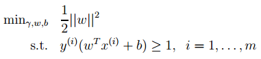
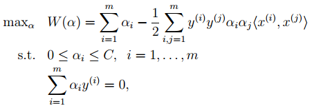
1. The optimal classification surface in SVM maximizes the geometric margin for all samples (why choose the maximum margin classifier? Please explain from a mathematical perspective; this has been asked during interviews for deep learning positions at NetEase. The answer is that there is a relationship between the geometric margin and the number of misclassifications of samples: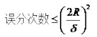 , where the denominator represents the distance from the sample to the classification margin, and R in the numerator is the longest vector value among all samples), that is:
Through a series of derivations, we can obtain the optimization of the following original objective:
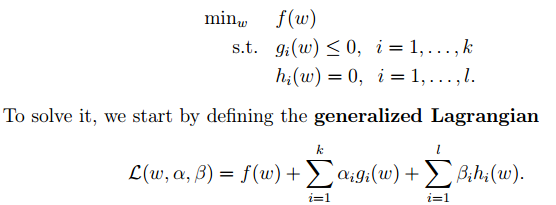
2. Next, let’s look at Lagrange theory:
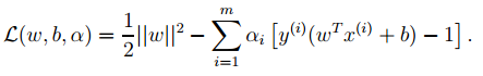
We can convert the optimization objective from 1 into Lagrange form (through various dual optimizations, KKT conditions), and finally the objective function becomes:
We only need to minimize the above objective function, where α is the Lagrange multiplier corresponding to the inequality constraint in the original optimization problem.
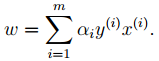
3. To derive the last objective function in 2 with respect to w and b, we get:
From the first equation above, we can see that if we optimize α, we can directly obtain w, thus determining the model parameters. The second equation can serve as a constraint condition for subsequent optimizations.
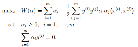
4. The last objective function in 2 can be transformed into optimizing the following objective function using dual optimization theory:
This function can be solved for α using common optimization methods, thus obtaining w and b.
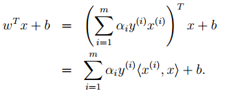
5. Theoretically, the simple theory of SVM should end here. However, one more point to add is that during prediction:
We can replace that angle bracket with a kernel function, which is also the reason SVM is often associated with kernel functions.
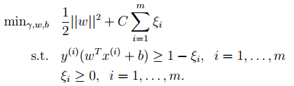
6. Finally, regarding the introduction of slack variables, the original optimization formula becomes:
The corresponding dual optimization formula is:
Compared to the previous one, α now has an upper bound.
SVM Algorithm Advantages:
1. Can be used for linear/non-linear classification, also applicable for regression;
2. Low generalization error;
4. Low computational complexity;
1. Sensitive to parameter and kernel function selection;
2. Original SVM is primarily adept at handling binary classification problems;
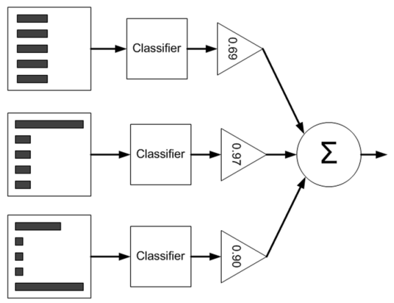
Taking Adaboost as an example, let’s first look at the flowchart of Adaboost:
From the diagram, we can see that during the training process, we need to train multiple weak classifiers (3 in the diagram), each weak classifier is trained using samples with different weights (5 training samples in the diagram). Each weak classifier contributes differently to the final classification result, which is output through a weighted average, with weights shown in the triangle in the diagram. So how are these weak classifiers and their corresponding weights trained?
Below is a simple example to illustrate: Assume there are 5 training samples, each with a dimension of 2. When training the first classifier, the weights of the 5 samples are all 0.2. Note that the sample weights and the corresponding weights α of the final trained weak classifiers are different; the sample weights are only used during the training process, while α is used in both the training and testing processes.
Now assume the weak classifier is a simple decision tree with one node, which will select one of the 2 attributes (assuming there are only 2 attributes) and compute the best value in that attribute for classification.
Adaboost’s simple version training process is as follows:
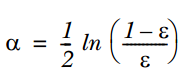
1. Train the first classifier, the sample weights D are equal. Through a weak classifier, predict the classification labels of these 5 samples (please refer to the example in the book, still machine learning in action) and compare with the true labels of the samples to obtain the error (i.e., misclassification). If a sample is predicted incorrectly, its corresponding error value is the weight of that sample; if classified correctly, the error value is 0. Finally, sum the error rates of the 5 samples to get ε.
2. Calculate the weight α of that weak classifier through ε, as follows:
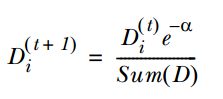
3. Use α to calculate the weight D of the training samples for the next weak classifier. If the corresponding sample is classified correctly, reduce the weight of that sample, as follows:
If the sample is classified incorrectly, increase that sample’s weight, as follows:
4. Loop through steps 1, 2, and 3 to continue training multiple classifiers, just with different D values.
Testing process is as follows:
Input a sample into each trained weak classifier, so each weak classifier corresponds to an output label, then that label is multiplied by the corresponding α, and finally, summing gives the sign of the predicted label value.
Advantages of Boosting Algorithms:
1. Low generalization error;
2. Easy to implement, high classification accuracy, with few parameters to tune;
4. Sensitive to outliers;
Based on clustering ideas, we can categorize:
1. Partition-based clustering:
K-means, k-medoids (finding a sample point to represent each category), CLARANS.
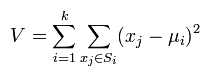
K-means minimizes the following expression:
K-means algorithm advantages:
(1) K-means is a classic algorithm for solving clustering problems, being simple and fast.
(2) It is relatively scalable and efficient for handling large datasets, with a complexity of about O(nkt), where n is the total number of objects, k is the number of clusters, and t is the number of iterations. Typically, k << n. This algorithm usually converges locally.
(3) The algorithm attempts to find k partitions that minimize the squared error function value. Clustering works well when the clusters are dense, spherical, or blob-like, and clearly distinguishable from each other.
(1) The k-means method can only be used when the average of the clusters is defined and is not suitable for some categorical data attributes.
(2) Requires the user to specify the number of clusters k in advance.
(3) Sensitive to initial values; different initial values may lead to different clustering results.
(4) Not suitable for discovering non-convex shaped clusters or clusters with significantly different sizes.
(5) Sensitive to noise and isolated point data; a small amount of such data can significantly affect the average.
2. Hierarchical clustering:
Bottom-up agglomerative methods, such as AGNES.
Top-down divisive methods, such as DIANA.
3. Density-based clustering: DBSACN, OPTICS, BIRCH (CF-Tree), CURE.
4. Grid-based methods: STING, WaveCluster.
5. Model-based clustering: EM, SOM, COBWEB.
Recommendation Systems: The implementation of recommendation systems mainly divides into content-based implementation and collaborative filtering implementation.
Content-based Implementation: The example of different people rating different movies can be seen as a standard regression problem, so each movie needs to extract a feature vector (the x value) in advance, and then model it for each user, with the ratings given by each user as the y value. Using these existing y ratings and movie feature values x, a regression model can be trained (the most common is linear regression).
Thus, it can predict the scores of movies that users have not rated. (It is worth noting that a regression model needs to be established for each user.)
From another perspective, it can also be to first specify each user’s preference for a certain movie (i.e., weight), then learn the features of each movie, and finally use regression to predict the scores of movies that have not been rated.
Of course, it can also optimize to obtain each user’s preferences for different types of movies and the features of each movie simultaneously.
Collaborative Filtering Implementation: Collaborative Filtering (CF) can be viewed as a classification problem or a matrix decomposition problem. Collaborative filtering is primarily based on the feature that each person’s preferences are similar; it does not rely on personal basic information.
For example, in the previous movie rating example, predicting the scores of movies that have not been rated relies solely on the scores that have been rated and does not need to learn the features of those movies.
SVD decomposes the matrix into the product of three matrices, as shown in the formula:
In the middle matrix, sigma is a diagonal matrix, and the values of the diagonal elements are the singular values of the Data matrix (note that singular values and eigenvalues are not the same), and they are already arranged from large to small. Even if the smaller singular values are removed, the original matrix can still be reconstructed well. As shown in the figure below:
, where the denominator represents the distance from the sample to the classification margin, and R in the numerator is the longest vector value among all samples), that is:
Through a series of derivations, we can obtain the optimization of the following original objective:
2. Next, let’s look at Lagrange theory:
We can convert the optimization objective from 1 into Lagrange form (through various dual optimizations, KKT conditions), and finally the objective function becomes:
We only need to minimize the above objective function, where α is the Lagrange multiplier corresponding to the inequality constraint in the original optimization problem.
3. To derive the last objective function in 2 with respect to w and b, we get:
From the first equation above, we can see that if we optimize α, we can directly obtain w, thus determining the model parameters. The second equation can serve as a constraint condition for subsequent optimizations.
4. The last objective function in 2 can be transformed into optimizing the following objective function using dual optimization theory:
This function can be solved for α using common optimization methods, thus obtaining w and b.
5. Theoretically, the simple theory of SVM should end here. However, one more point to add is that during prediction:
We can replace that angle bracket with a kernel function, which is also the reason SVM is often associated with kernel functions.
6. Finally, regarding the introduction of slack variables, the original optimization formula becomes:
The corresponding dual optimization formula is:
Compared to the previous one, α now has an upper bound.
SVM Algorithm Advantages:
1. Can be used for linear/non-linear classification, also applicable for regression;
2. Low generalization error;
4. Low computational complexity;
1. Sensitive to parameter and kernel function selection;
2. Original SVM is primarily adept at handling binary classification problems;
Taking Adaboost as an example, let’s first look at the flowchart of Adaboost:
From the diagram, we can see that during the training process, we need to train multiple weak classifiers (3 in the diagram), each weak classifier is trained using samples with different weights (5 training samples in the diagram). Each weak classifier contributes differently to the final classification result, which is output through a weighted average, with weights shown in the triangle in the diagram. So how are these weak classifiers and their corresponding weights trained?
Below is a simple example to illustrate: Assume there are 5 training samples, each with a dimension of 2. When training the first classifier, the weights of the 5 samples are all 0.2. Note that the sample weights and the corresponding weights α of the final trained weak classifiers are different; the sample weights are only used during the training process, while α is used in both the training and testing processes.
Now assume the weak classifier is a simple decision tree with one node, which will select one of the 2 attributes (assuming there are only 2 attributes) and compute the best value in that attribute for classification.
Adaboost’s simple version training process is as follows:
1. Train the first classifier, the sample weights D are equal. Through a weak classifier, predict the classification labels of these 5 samples (please refer to the example in the book, still machine learning in action) and compare with the true labels of the samples to obtain the error (i.e., misclassification). If a sample is predicted incorrectly, its corresponding error value is the weight of that sample; if classified correctly, the error value is 0. Finally, sum the error rates of the 5 samples to get ε.
2. Calculate the weight α of that weak classifier through ε, as follows:
3. Use α to calculate the weight D of the training samples for the next weak classifier. If the corresponding sample is classified correctly, reduce the weight of that sample, as follows:
If the sample is classified incorrectly, increase that sample’s weight, as follows:
4. Loop through steps 1, 2, and 3 to continue training multiple classifiers, just with different D values.
Testing process is as follows:
Input a sample into each trained weak classifier, so each weak classifier corresponds to an output label, then that label is multiplied by the corresponding α, and finally, summing gives the sign of the predicted label value.
Advantages of Boosting Algorithms:
1. Low generalization error;
2. Easy to implement, high classification accuracy, with few parameters to tune;
4. Sensitive to outliers;
Based on clustering ideas, we can categorize:
1. Partition-based clustering:
K-means, k-medoids (finding a sample point to represent each category), CLARANS.
K-means minimizes the following expression:
K-means algorithm advantages:
(1) K-means is a classic algorithm for solving clustering problems, being simple and fast.
(2) It is relatively scalable and efficient for handling large datasets, with a complexity of about O(nkt), where n is the total number of objects, k is the number of clusters, and t is the number of iterations. Typically, k << n. This algorithm usually converges locally.
(3) The algorithm attempts to find k partitions that minimize the squared error function value. Clustering works well when the clusters are dense, spherical, or blob-like, and clearly distinguishable from each other.
(1) The k-means method can only be used when the average of the clusters is defined and is not suitable for some categorical data attributes.
(2) Requires the user to specify the number of clusters k in advance.
(3) Sensitive to initial values; different initial values may lead to different clustering results.
(4) Not suitable for discovering non-convex shaped clusters or clusters with significantly different sizes.
(5) Sensitive to noise and isolated point data; a small amount of such data can significantly affect the average.
2. Hierarchical clustering:
Bottom-up agglomerative methods, such as AGNES.
Top-down divisive methods, such as DIANA.
3. Density-based clustering: DBSACN, OPTICS, BIRCH (CF-Tree), CURE.
4. Grid-based methods: STING, WaveCluster.
5. Model-based clustering: EM, SOM, COBWEB.
Recommendation Systems: The implementation of recommendation systems mainly divides into content-based implementation and collaborative filtering implementation.
Content-based Implementation: The example of different people rating different movies can be seen as a standard regression problem, so each movie needs to extract a feature vector (the x value) in advance, and then model it for each user, with the ratings given by each user as the y value. Using these existing y ratings and movie feature values x, a regression model can be trained (the most common is linear regression).
Thus, it can predict the scores of movies that users have not rated. (It is worth noting that a regression model needs to be established for each user.)
From another perspective, it can also be to first specify each user’s preference for a certain movie (i.e., weight), then learn the features of each movie, and finally use regression to predict the scores of movies that have not been rated.
Of course, it can also optimize to obtain each user’s preferences for different types of movies and the features of each movie simultaneously.
Collaborative Filtering Implementation: Collaborative Filtering (CF) can be viewed as a classification problem or a matrix decomposition problem. Collaborative filtering is primarily based on the feature that each person’s preferences are similar; it does not rely on personal basic information.
For example, in the previous movie rating example, predicting the scores of movies that have not been rated relies solely on the scores that have been rated and does not need to learn the features of those movies.
SVD decomposes the matrix into the product of three matrices, as shown in the formula:
In the middle matrix, sigma is a diagonal matrix, and the values of the diagonal elements are the singular values of the Data matrix (note that singular values and eigenvalues are not the same), and they are already arranged from large to small. Even if the smaller singular values are removed, the original matrix can still be reconstructed well. As shown in the figure below:
 Where m represents the number of products, and n represents the number of users; each row of the U matrix represents the attributes of the product. Now, by reducing the dimensionality of the U matrix (taking the darker part), each product’s attributes can be represented in a lower dimension (assumed to be k dimensions). When a new user’s product recommendation vector X arrives, it can be represented as a k-dimensional vector according to the formula X’*U1*inv(S1), and then find the most similar user in V’ (similarity measurement can use cosine formula, etc.), and recommend based on that user’s ratings (mainly recommending those products that new users have not rated).
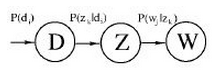
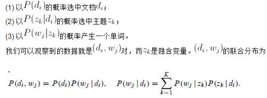
pLSA: Developed from LSA, where the early implementation of LSA was mainly through SVD decomposition. The model diagram of pLSA is as follows:
The meanings of the formulas are as follows:
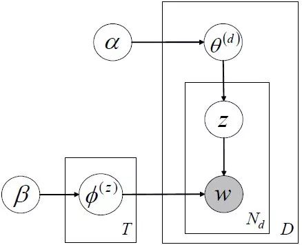
LDA topic model, probability graph as follows:
Unlike pLSA, LDA assumes many prior distributions, and the prior distribution of general parameters is usually assumed to be a Dirichlet distribution, the reason being that the conjugate distribution has the same form for prior and posterior probabilities.
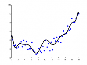
GDBT: GBDT (Gradient Boosting Decision Tree), also known as MART (Multiple Additive Regression Tree), is widely used internally at Alibaba (thus may be asked during algorithm job interviews at Alibaba). It is an iterative decision tree algorithm,composed of multiple decision trees, where the output results of all trees sum up to the final answer.
It was recognized from its inception alongside SVM as an algorithm with strong generalization capabilities. In recent years, it has gained attention for being used as a machine learning model for search ranking.
GBDT is a regression tree, not a classification tree. Its core is that each tree learns from the residuals of all previous trees. To prevent overfitting, boosting is also added, similar to Adaboost.
Regularization serves to:
1. Make numerical solutions easier to obtain;
2. Be more stable when the number of features is too large;
3. Control the complexity of the model and smoothness. The smaller and smoother the target function’s complexity, the stronger its generalization capability. Adding a regularization term can reduce the complexity of the target function and make it smoother.
4. Reduce the parameter space; the smaller the parameter space, the lower the complexity.
5. The smaller the coefficients, the simpler the model; the simpler the model, the stronger its generalization capability (as explained by Ng at a macro level).
6. Can be seen as a Gaussian prior on weights.
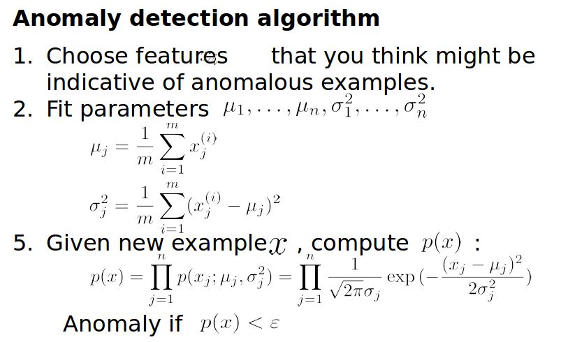
Outlier Detection: Outlier detection can estimate the density function of samples; for new samples, directly calculate their density, and if the density value is below a certain threshold, it indicates that the sample is an outlier. The density function is generally modeled using a multi-dimensional Gaussian distribution.
If the sample has n dimensions, each dimension’s features can be considered to follow a Gaussian distribution. Even if these features do not visually conform to a Gaussian distribution, mathematical transformations can be applied to make them appear Gaussian, such as x=log(x+c), x=x^(1/c), etc. The algorithm flow for outlier detection is as follows:
The ε is also obtained through cross-validation, meaning that in outlier detection, the learning of p(x) is unsupervised, while the learning of the parameter ε is supervised. Why not use ordinary supervised methods entirely (i.e., treat it as a standard binary classification problem)?
The main reason is that in outlier detection, the number of outlier samples is very small while the number of normal samples is very large, making it insufficient to learn good parameters for the outlier behavior model, as the new incoming outlier samples may completely differ from the patterns in the training samples.
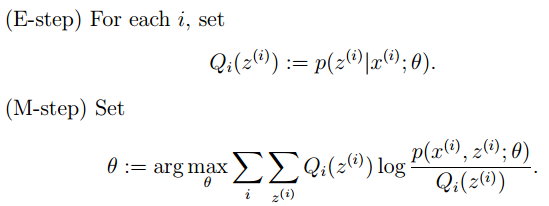
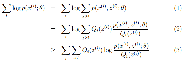
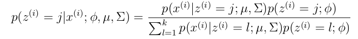
EM Algorithm: Sometimes, because the generation of samples is related to latent variables (latent variables are unobservable), the model parameters are generally estimated using maximum likelihood estimation. Since it involves latent variables, it is impossible to derive the likelihood function parameters directly; we can use the EM algorithm to estimate the model parameters (the number of parameters may be multiple).
EM algorithm generally consists of 2 steps:
E step: Select a set of parameters and calculate the conditional probability of the latent variables under those parameters;
M step: Combine the conditional probabilities of the latent variables obtained in the E step to maximize the lower bound of the likelihood function (essentially some expected function).
Repeat the above 2 steps until convergence, as shown in the formula:
The derivation of the lower bound function in the M step is as follows:
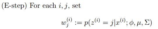
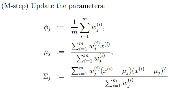
A common example of the EM algorithm is the GMM model, where each sample may be generated by k Gaussians, but the probability of being generated by each Gaussian differs. Therefore, each sample corresponds to a Gaussian distribution (one of k), and the latent variable at this time is the Gaussian distribution corresponding to each sample.
The E step formula for GMM is as follows (calculating the probability of each sample corresponding to each Gaussian):
More specifically, the calculation formula is:
The M step formula is as follows (calculating the weights, means, and variances of each Gaussian):
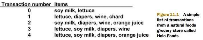
Apriori is one of the earlier methods in association analysis, primarily used to mine frequent itemsets. Its ideas are:
1. If a project set is not frequent, then any project set containing it cannot be frequent;
2. If a project set is frequent, then any non-empty subset of it must also be frequent;
Apriori requires scanning the project table multiple times, starting from one project, eliminating those that are not frequent, obtaining a set called L, and then self-combining each element in L to generate a set with one more project than the last scan, called C, followed by another scan to eliminate non-frequent projects, and repeating…
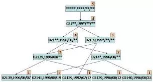
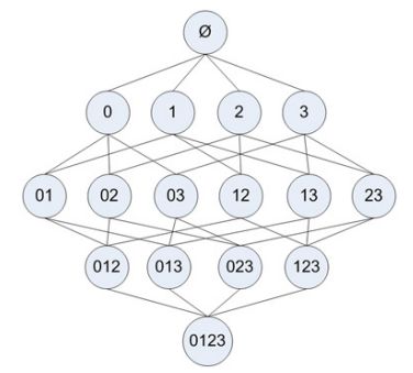
Consider the following example of an element project table:
If in each step we do not eliminate non-frequent item sets, the scanning process tree structure is as follows:
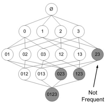
In some process, a non-frequent item set may appear, which will be eliminated (shadowed):
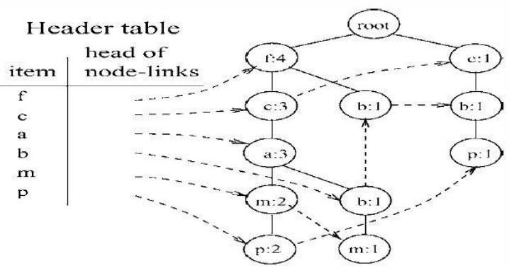
FP Growth is a more efficient frequent item mining method than Apriori, requiring only two scans of the project table. The first scan obtains the frequency of each project, removing those that do not meet the support requirement, and sorts the remaining items. The second scan constructs an FP-Tree (frequent-pattern tree).
The subsequent work is to mine on the FP-Tree, for example, given the following table:
It corresponds to the FP_Tree as follows:
Then, starting from the least frequent single item P, find P’s conditional pattern base, and construct the FP_Tree for P’s conditional pattern base in the same way, then find the frequent item sets that include P on this tree.
Subsequently, mine frequent item sets from the conditional pattern bases of m, b, a, c, f; some items may require recursive mining, which can be quite tedious, such as the m node.
Where m represents the number of products, and n represents the number of users; each row of the U matrix represents the attributes of the product. Now, by reducing the dimensionality of the U matrix (taking the darker part), each product’s attributes can be represented in a lower dimension (assumed to be k dimensions). When a new user’s product recommendation vector X arrives, it can be represented as a k-dimensional vector according to the formula X’*U1*inv(S1), and then find the most similar user in V’ (similarity measurement can use cosine formula, etc.), and recommend based on that user’s ratings (mainly recommending those products that new users have not rated).
pLSA: Developed from LSA, where the early implementation of LSA was mainly through SVD decomposition. The model diagram of pLSA is as follows:
The meanings of the formulas are as follows:
LDA topic model, probability graph as follows:
Unlike pLSA, LDA assumes many prior distributions, and the prior distribution of general parameters is usually assumed to be a Dirichlet distribution, the reason being that the conjugate distribution has the same form for prior and posterior probabilities.
GDBT: GBDT (Gradient Boosting Decision Tree), also known as MART (Multiple Additive Regression Tree), is widely used internally at Alibaba (thus may be asked during algorithm job interviews at Alibaba). It is an iterative decision tree algorithm,composed of multiple decision trees, where the output results of all trees sum up to the final answer.
It was recognized from its inception alongside SVM as an algorithm with strong generalization capabilities. In recent years, it has gained attention for being used as a machine learning model for search ranking.
GBDT is a regression tree, not a classification tree. Its core is that each tree learns from the residuals of all previous trees. To prevent overfitting, boosting is also added, similar to Adaboost.
Regularization serves to:
1. Make numerical solutions easier to obtain;
2. Be more stable when the number of features is too large;
3. Control the complexity of the model and smoothness. The smaller and smoother the target function’s complexity, the stronger its generalization capability. Adding a regularization term can reduce the complexity of the target function and make it smoother.
4. Reduce the parameter space; the smaller the parameter space, the lower the complexity.
5. The smaller the coefficients, the simpler the model; the simpler the model, the stronger its generalization capability (as explained by Ng at a macro level).
6. Can be seen as a Gaussian prior on weights.
Outlier Detection: Outlier detection can estimate the density function of samples; for new samples, directly calculate their density, and if the density value is below a certain threshold, it indicates that the sample is an outlier. The density function is generally modeled using a multi-dimensional Gaussian distribution.
If the sample has n dimensions, each dimension’s features can be considered to follow a Gaussian distribution. Even if these features do not visually conform to a Gaussian distribution, mathematical transformations can be applied to make them appear Gaussian, such as x=log(x+c), x=x^(1/c), etc. The algorithm flow for outlier detection is as follows:
The ε is also obtained through cross-validation, meaning that in outlier detection, the learning of p(x) is unsupervised, while the learning of the parameter ε is supervised. Why not use ordinary supervised methods entirely (i.e., treat it as a standard binary classification problem)?
The main reason is that in outlier detection, the number of outlier samples is very small while the number of normal samples is very large, making it insufficient to learn good parameters for the outlier behavior model, as the new incoming outlier samples may completely differ from the patterns in the training samples.
EM Algorithm: Sometimes, because the generation of samples is related to latent variables (latent variables are unobservable), the model parameters are generally estimated using maximum likelihood estimation. Since it involves latent variables, it is impossible to derive the likelihood function parameters directly; we can use the EM algorithm to estimate the model parameters (the number of parameters may be multiple).
EM algorithm generally consists of 2 steps:
E step: Select a set of parameters and calculate the conditional probability of the latent variables under those parameters;
M step: Combine the conditional probabilities of the latent variables obtained in the E step to maximize the lower bound of the likelihood function (essentially some expected function).
Repeat the above 2 steps until convergence, as shown in the formula:
The derivation of the lower bound function in the M step is as follows:
A common example of the EM algorithm is the GMM model, where each sample may be generated by k Gaussians, but the probability of being generated by each Gaussian differs. Therefore, each sample corresponds to a Gaussian distribution (one of k), and the latent variable at this time is the Gaussian distribution corresponding to each sample.
The E step formula for GMM is as follows (calculating the probability of each sample corresponding to each Gaussian):
More specifically, the calculation formula is:
The M step formula is as follows (calculating the weights, means, and variances of each Gaussian):
Apriori is one of the earlier methods in association analysis, primarily used to mine frequent itemsets. Its ideas are:
1. If a project set is not frequent, then any project set containing it cannot be frequent;
2. If a project set is frequent, then any non-empty subset of it must also be frequent;
Apriori requires scanning the project table multiple times, starting from one project, eliminating those that are not frequent, obtaining a set called L, and then self-combining each element in L to generate a set with one more project than the last scan, called C, followed by another scan to eliminate non-frequent projects, and repeating…
Consider the following example of an element project table:
If in each step we do not eliminate non-frequent item sets, the scanning process tree structure is as follows:
In some process, a non-frequent item set may appear, which will be eliminated (shadowed):
FP Growth is a more efficient frequent item mining method than Apriori, requiring only two scans of the project table. The first scan obtains the frequency of each project, removing those that do not meet the support requirement, and sorts the remaining items. The second scan constructs an FP-Tree (frequent-pattern tree).
The subsequent work is to mine on the FP-Tree, for example, given the following table:
It corresponds to the FP_Tree as follows:
Then, starting from the least frequent single item P, find P’s conditional pattern base, and construct the FP_Tree for P’s conditional pattern base in the same way, then find the frequent item sets that include P on this tree.
Subsequently, mine frequent item sets from the conditional pattern bases of m, b, a, c, f; some items may require recursive mining, which can be quite tedious, such as the m node.
-END-

关注【中科院计算所培训中心】
阅读更多精彩内容
▽▽▽
点分享

点点赞

点在看