Comprehensive Introduction to Convolutional Neural Networks

Introduction: AI, CNN Algorithm, Hilbert, Feynman, 577

What is the hottest and most well-known core mathematical algorithm of AI today? The answer is the “Convolutional Neural Network Algorithm”.

Mathematics is the foundation of all science and technology, and the Convolutional Neural Network algorithm is no exception. It is the basis and core of almost all AI products and applications. Without it, none of the AI products in this wave of AI fever would exist.

So what exactly is a Convolutional Neural Network (hereinafter referred to as CNN for convenience)? What do “convolution”, “neural”, and “network” mean? How does it achieve image recognition?

Today, I will share my understanding of these concepts in the most down-to-earth language possible.

Mathematics is the ceiling of software; I hope this helps everyone achieve the small goal of earning over ten thousand a month while sleeping, and not to be a 577 during interviews.

Feynman said: The process of sharing and organizing easy-to-understand language is also a process of deeply and accurately understanding and learning content, and improving oneself. So thank you for clicking on this article about mathematical algorithms. As a die-hard fan of Hilbert and Feynman, I will also avoid presenting a series of high-energy mathematical formulas.

The article is quite long, and to avoid it falling apart and to ensure clarity, I will use my understanding of the following 13 key terms as the main line of the article: Convolution Kernel, Convolution Algorithm, Convolution, Convolution Layer (collectively known as the four brothers of the convolution family), Filter, Feature Detector, Pooling Layer, Fully Connected Layer, Summation, Weight Coefficient, Flattening, Deep Learning, Overfitting Phenomenon, Perceptron. If you understand these 13 terms, you will have grasped 80-90% of the CNN algorithm.

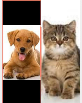
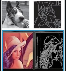
Who are the eldest, second, and third brothers of the convolution family?

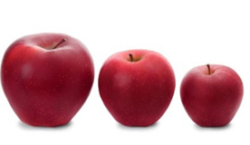
Starting from the division of apples into sizes…

The eldest, second, and third brothers are: the Eldest Brother Convolution Kernel, the Second Brother Convolution Algorithm, and the Third Brother Convolution: “The Convolution Kernel is a small matrix, the Convolution Algorithm is as the name suggests an algorithm, and Convolution is a numerical value (real number). Using the ‘Convolution Kernel’ and another small matrix of the same size to perform ‘Convolution Operation’, the result will yield a numerical value, which is called Convolution.”

Did you not understand? It’s okay if you didn’t; just continue reading, and you will understand by the end of this section.

Let’s first talk about the Eldest Brother ‘Convolution Kernel’. Foodies know that fruit shop owners online usually classify their fruits into large, medium, and small sizes, with large fruits being the most expensive and small fruits the cheapest.

So how do shop owners classify large, medium, and small fruits? They don’t measure each fruit one by one with a ruler, which would be too slow. Instead, they find a piece of cardboard with two holes of different sizes. If a fruit cannot pass through the large hole, it is classified as a large fruit; if it can pass through the small hole, it is classified as a small fruit; if it can pass through the large hole but not the small hole, it is classified as a medium fruit.

These two holes are called two “Filters”; please remember this term — “Filter”. It is the alias of the Eldest Brother ‘Convolution Kernel’ and a name that better reveals the essence of graphics. For ease of understanding, we will continue to use the alias “Filter” in the following text.

Next, let’s consider a slightly more complex example: how to differentiate between a dog and a cat? Cats have pointed ears, while dogs have round ears. How does a computer differentiate whether an animal in a picture is a cat or a dog (assuming there is only one animal in the photo)? Should it find the ears first and then measure the angles? That’s too slow.

How can we speed this up? We can still use the ‘Filter’ method: directly find the contour curve of a dog’s ear, as shown in the lower right corner of Figure 1, and cut a slit in a piece of cardboard that matches this curve.

Then, move the cardboard over the photographic image. If a segment of the contour line in the photo matches the curve of the slit very closely, we classify this photo as a dog; if no area matches the contour line of a dog’s ear, we classify it as a cat.

This slit in the curve is a ‘Filter’, and any part that does not match this curve is ignored, leaving only the parts that match its shape as the basis for classification.

This contour line of a dog’s ear can also be considered a feature of the dog, distinguishing it from a cat, so the Eldest Brother ‘Convolution Kernel’ has gained a third name: ‘Feature Detector’.

In the future, for ease of writing and to help everyone understand the context, I will alternate between using the terms ‘Filter’, ‘Feature Detector’, and ‘Convolution Kernel’. Remember that these three terms refer to the same thing; ‘Convolution Kernel’ has a more algebraic meaning, while the other two have more graphical meanings.

Of course, AI software is not human; it does not move a piece of cardboard over a photographic image. So how does it work?

Please look at the 7×7 small matrix in the lower left corner of Figure 1. It represents the algebraic meaning of the Eldest Brother ‘Convolution Kernel’. Each element of the matrix corresponds to a pixel in the image. Pay attention to the gray part, where the element value is 30; the curve formed by these points corresponds exactly to the black curve in the lower right corner.

Everyone knows that an electronic image is essentially a large matrix, for example, 1024×768, where each element of the matrix corresponds to a pixel.

Now, let the 7×7 small matrix in the lower right corner move pixel by pixel from left to right and top to bottom across the large matrix of the photo (see the animated diagram in Figure 2). This effect is equivalent to a person moving a piece of cardboard over a physical photograph.

Figure 1 The Filter (Convolution Kernel, Feature Detector) of a Dog’s Ear

Some smart friends might ask: “When the Eldest Brother ‘Convolution Kernel’ small matrix moves pixel by pixel over the large matrix, how does the software determine whether there is a highly matching curve at this position?”

At this point, we need to rely on the Second Brother ‘Convolution Algorithm’. So how does this Second Brother operate? It is simply “multiplying a matrix (the Convolution Kernel) with another matrix of the same size pixel by pixel, and then summing these products. The final sum is called ‘Convolution’ (the Third Brother).”

To help everyone understand this concept, please refer to the animated diagram in Figure 2.

Figure 2 Animated demonstration of Convolution Algorithm

So what effect does this Second Brother ‘Convolution Algorithm’ have?

Please look at the 7×7 small matrix of the Eldest Brother ‘Convolution Kernel’ in the lower right corner. Apart from the part that resembles the curve of a cartoon dog’s ear, which has a value of 30, all other places are 0.

This means that when it performs convolution with a certain 7×7 small matrix on the image, if the corresponding area on the image matrix has values of 255, then the convolution of these two small matrices will be 0 + 7×30×255 = 53550. The 7 here is because the number of points with a value of 30 is 7, and the 0 is because all other elements in the filter are zero.

53550 is the maximum convolution value for our “cartoon dog’s ear filter”. This maximum value means that “within this 7×7 small area of the image, there is a pure white curve shape that completely matches the filter’s cat curve”.

However, if you directly move the small matrix of the filter over the colorful cartoon dog image and calculate convolution at each point, you will find that the convolution value at the white background area is also 53550. This does not achieve the goal of finding the feature curve in the image.

How do we solve this problem? We preprocess the colorful cartoon dog image first, quickly outlining the boundary lines where the color changes and keeping only the boundary lines, turning the rest into black, as shown in the upper right corner.

Using the small matrix from the lower left corner to perform convolution on the preprocessed cartoon dog image will ensure that only areas matching the feature curve yield a convolution value of 53550.

In fact, not only the cartoon dog in Figure 1, but all AI software based on CNN typically processes image problems by first identifying edges and retaining only the edges. For example, in Figure 3, the cartoon dog and the beautiful woman; remember that beautiful woman, you will see her frequently if you successfully apply for a job.

Finding the edge line is just a preprocessing step before the CNN algorithm officially starts. To avoid taking away from the main topic, I won’t elaborate on this here. Interested friends can search for Sobel filters on their own.

Figure 3 Extracting Image Edges

Some friends may ask: “Chao Mo Jun, your method is not accurate. The curve of the cartoon dog’s ear cannot be found in most real dog photos! Not to mention, in the edge image of the big dog in Figure 3, it cannot be found. Besides the big dog in Figure 3, many dogs also have pointed ears, like Siberian Huskies; cats also have droopy ears, like Scottish Fold cats.”

What should we do in this case? We need to find a curve that is commonly found on dogs but not on cats as a ‘Feature Detector’, such as the outline of a long mouth, and use two ‘Feature Detectors’ to improve accuracy compared to using just one.

For a more complex example, how do we differentiate between over 100 breeds of dogs? In this case, using only the ear contour line and the long mouth contour line as “Feature Detectors” is insufficient; we also need the contour line of the tail and forehead to identify more accurately.

Figure 4 Dog Breed Rally

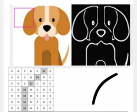
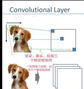
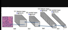
Next, let’s look at the Fourth Brother of the Convolution Family, the ‘Convolution Layer’

Understanding the four brothers means you’ve succeeded halfway

The previous section mentioned the method of using multiple ‘Feature Detectors’ simultaneously.

“If multiple Feature Detectors scan the image, does this mean that the Convolution Algorithm will need to run multiple times? These multiple runs and Feature Detectors (also known as Convolution Kernels, Filters) are collectively referred to as ‘Convolution Layer’. The number of images generated by a Convolution Layer corresponds to the number of Feature Detectors used.”

Please see the diagram below, where there are ‘Ear Curve’, ‘Nose Curve’, and ‘Back Curve’ as three Feature Detectors. After processing the image with these three Feature Detectors, one image becomes three images.

Figure 5 Three Feature Detectors Transform One Image into Three Images

One image corresponds to one Feature Detector

Alright, by now, you should know what ‘Convolution’, ‘Convolution Algorithm’, ‘Convolution Kernel’, and ‘Convolution Layer’ are, and you can say you have grasped the main essence of CNN. If you are applying for a regular engineer position, even the most arrogant interviewer will give you a “not bad” evaluation in their mind.

‘Neural’ means what? A misleading term.

This is a misleading term, a term that confuses people, and a term that can mislead. If you want to learn AI, don’t pay attention to this term. I was misled by this term at first, wasting at least half a year of my precious time.

The inventor of the CNN algorithm (or possibly the commercial promotion team behind him) claims that this algorithm is as intelligent as the human brain, and its structure and the principles of generating intelligence are similar to the “neural network” in the brain. This is nonsense. Not to mention that whether advanced human intelligence, such as inductive reasoning and imagination, comes from the brain is still not determined; this is merely a guess or a hypothesis (most of my coding colleagues believe that the brain is equivalent to the ‘south bridge’ on a computer motherboard, which only manages external devices).

Even if it truly comes from the neural network in the brain, there is no similarity between CNN and neural networks.

In fact, the so-called ‘neurons’ refer to the vectors produced when the CNN algorithm is nearing completion. The elements on the vector are also called ‘Perceptrons’.

To run fast, a horse must not only eat grass but also avoid pits on the road; otherwise, if its leg steps into a pit, it may break. The term “neuron” is a pit; I advise you to avoid this pit. Because ‘Neural’, ‘Neuron’, and ‘Neural Network’ are purely misleading, I did not include them in the 13 key terms.

Comprehensive Introduction to Convolutional Neural Networks

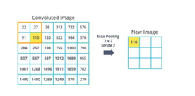
Besides ‘Convolution Layer’, what are the other two layers?

What does ‘Network’ mean in CNN?

We have already discussed the meanings of ‘Convolution’ and ‘Neural’; now let’s talk about the term ‘Network’.

This term, when paired with the bad kid ‘Neural’, is misleading. However, if used alone, it has some meaning. Before explaining its true meaning, let me first introduce four other key terms: ‘Pooling Layer’, ‘Fully Connected Layer’, ‘Flattening’, and ‘Weight Coefficient’ (the Weight Coefficient is also very important; everyone must remember it well).

The ‘Pooling Layer’ mainly serves to reduce the size of the image or the number of pixels to decrease the overall computation of the system. For example, in the image below, a 6×6 matrix is transformed into a 3×3 matrix, retaining only the maximum value within a 2×2 small area while ignoring the rest, resulting in a 6×6 becoming a 3×3.

Figure 6 Example of Pooling Layer

Typically, ‘Pooling’ and ‘Convolution Layer’ run in an iterative loop, meaning that first, the image undergoes convolution processing, then the Pooling Layer reduces the size of the convolved image, followed by another set of filters, and then the image is processed again by the Convolution Layer, and so on… This iterative process continues multiple times, resulting in a set of relatively small images. The number of images corresponds to the product of the number of filters used in each convolution layer. For example, if the first convolution layer uses 64 filters, the second uses 8 filters, and the third uses 4 filters, then the total number of images generated after three iterations would be 64×8×4=2048 images.

Figure 7 Two Iterations of Convolution Layer and Pooling Layer

The image size becomes smaller, and the number of images increases.

Next, the ‘Fully Connected Layer’ will make its appearance. From a coder’s perspective, it would be more reasonable to call it the ‘Summation Layer’.

Everyone knows that an image is a matrix. After the last pooling layer, the number of matrices corresponds to the number of images. The task of the ‘Fully Connected Layer’ is to convert multiple matrices into a vector, which means flattening the two-dimensional matrix into a one-dimensional vector.

How is this flattening done? It involves two rounds of ‘Summation’. The first round sums the values of each pixel in the processed image. What is the practical significance of this step?

Taking the dog’s ear curve as an example, the dog’s ear can be in any position in the image. The purpose of the first ‘Summation’ is: ‘I don’t care where the dog’s ear curve is; I just want the dog’s ear curve.’ The larger the sum, the greater the likelihood that the image contains a dog’s ear.

After performing ‘Summation’ on n images, we will obtain n sums. If placed in a vector, it becomes a vector with n elements. How do we convert this vector into a single value?

That is done through a second ‘Summation’. We find a vector with n elements (for ease of writing, let’s call it vector A) that is perpendicular to the previous n-element vector (let’s call it vector B). Multiplying these two vectors will yield a single value (for convenience, let’s call it ‘V_dog’).

How do we fill in the values of the elements in vector B? That is where the ‘Weight Coefficient’ comes in. The practical significance of this ‘Weight Coefficient’ is that while dogs have various ‘Feature Detectors’, the weights of different features are not the same when determining whether an image depicts a dog. For instance, ‘curled tail’ is more significant than ‘droopy ear curve’; if the image shows a curled tail, it must be a dog, not a cat.

Conversely, the droopy ear curve is different; among dogs, there are also upright-eared breeds like Siberian Huskies, and among cats, there are also droopy-eared breeds like Scottish Fold cats. Thus, we can set the weight coefficient of the ‘curled tail feature detector’ to 20 and the weight coefficient of the ‘droopy ear curve feature detector’ to 10.

At this point, we have transformed the question of whether an image depicts a dog into a ‘single value’. Similarly, we can find another vector B’ for cats, assigning different weight coefficients, such as setting the curled tail weight coefficient to 0 and the droopy ear weight coefficient to 2. By multiplying vector B’ with vector A, we can also obtain a value ‘V_cat’. We can then place ‘V_cat’ and ‘V_dog’ into a vector containing these two elements; this two-element vector is the output of the ‘Fully Connected Layer’.

‘Fully Connected’ means that all pixel values from all images are summed together. ‘All’ means all; all images, all pixel values, and ‘Connected’ essentially means summation.

All images, all pixels, all connections are like a network. This is the origin of the term ‘network’ in ‘Convolutional Neural Network’, as ‘network’ is not entirely accurate (it only appears somewhat similar), which can lead to misunderstanding, so I did not include it in the 13 keywords.

Although I do not agree with the term ‘Neural’, believing it to be misleading.

However, to communicate with interviewers, we still need to discuss what ‘neurons’ refer to in CNN. They refer to the aforementioned ‘V_dog’, ‘V_cat’, etc. If we need to distinguish not only between cats and dogs but also between pigs, sheep, and chickens, the output of the fully connected layer would be a vector containing five elements, where the neurons represent ‘V_dog’, ‘V_cat’, ‘V_pig’, ‘V_sheep’, and ‘V_chicken’. This vector is also known as ‘Perceptron’, which is actually a more accurate term.

Once we have a vector composed of ‘Perceptrons’, the subsequent work is simple: we normalize ‘V_dog’ and ‘V_cat’ to convert them into probability values. For example, if V_dog=200 and V_cat=3, the probability that the image is a dog is 200÷(200+3)=98.5%, while the probability that it is a cat is 1.5%.

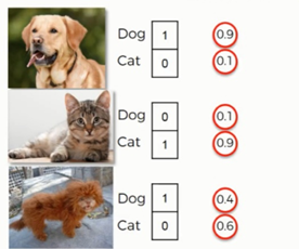
CNN’s Second Half: What is Learned in Deep Learning?

What is the fundamental flaw of CNN?

In this section, we will discuss another commonly used term in AI or CNN: ‘Deep Learning’. Other software coders can directly use their code after it is completed without bugs.

However, AI software based on CNN is different. After the coder completes the code without bugs, that only completes the first half. This means that even if the coder finishes, the software cannot be used; it still needs to learn and be trained before it can be used.

What does it learn and train on? Do you remember the two words I insisted you remember earlier? One is ‘Filter’ (which is a small matrix), and the other is ‘Weight Coefficient’ (which is a number). The learning process involves continuously adjusting these ‘Filters’ and ‘Weight Coefficients’.

When the coder first delivers it, the Filters and Weight Coefficients are very inaccurate, and the accuracy of identifying whether an image is a cat or a dog is less than 0.001%. At this time, when given an image and told the answer (i.e., whether the image is a cat or a dog), the AI software will correct the Filters and Weight Coefficients until it finds a set of Filters and Weight Coefficients that yield a conclusion close to or identical to the correct answer.

Then, when given another image with a known answer, the group of Filters and Weight Coefficients obtained from the previous image may not be accurate for this new image, so the AI software will again correct the Filters and Weight Coefficients (note that adjusting the Filters also includes modifying existing Filters and potentially adding new ones).

Next, when given a third image with a known answer, it will again adjust the Filters and Weight Coefficients. This process continues repeatedly. After thousands of images, the AI will obtain a reasonable set of Filters and Weight Coefficients, allowing it to accurately identify whether an image depicts a cat or a dog. For more complex problems, such as identifying cats, dogs, sheep, pigs, and chickens, it may require tens of thousands of images with known answers for the AI software to learn.

This learning process has three characteristics:

1. Generally speaking, the larger the training volume, the higher the accuracy.

This is why, in the AI machine translation field, large language translations, such as English-Chinese translation, have high accuracy due to the large training volume. However, small languages struggle; for example, Armenian to Chinese has lower accuracy due to insufficient training volume.

2. The speed of learning progress is initially fast but slows down over time.

3. Regardless of how large the training volume is, accuracy can never reach 100%. This brings us to the key term “Overfitting Phenomenon”. Even if you provide it with 100 million images to learn from, it may still make mistakes on the 100 million and first image.“Overfitting Phenomenon” is a fundamental and inherent flaw of AI software based on the CNN algorithm that cannot be eliminated.

For this reason, AI cannot replace human drivers. Recognizing whether an image depicts a cat or a dog with a 1% error margin is acceptable, but making mistakes while driving can lead to catastrophic outcomes.Therefore, current AI cars are only allowed to drive slowly on dedicated scenic routes.

Conclusion

Finally, let’s review the CNN terms and concepts mentioned in this article.

Understanding the 13 key terms: Convolution Kernel, Convolution Algorithm, Convolution, Convolution Layer (collectively known as the four brothers of the convolution family), Filter, Feature Detector (two aliases of the Convolution Kernel), Pooling Layer, Fully Connected Layer, Summation, Weight Coefficient, Flattening, Deep Learning, Overfitting Phenomenon, Perceptron.

There are also three misleading terms that you should be aware of for communication with interviewers: Neural, Neuron, Neural Network.

Remember, understanding these concepts is more important than just memorizing them. Don’t do mathematics just for the sake of mathematics. I believe you can become a little champion in interviews and achieve the small goal of earning over ten thousand after tax.

In Closing

If you think this article is well-written, please support me. Especially this set of “The Journey of Physics: 54 Physicists Who Shone in Human History”.

54 great figures in the history of physics are waiting for you to explore.

If you want to learn more, please pay attention to this set of “The Journey of Physics: 54 Physicists Who Shone in Human History”.

Buy now, and for just an additional 1 yuan, receive a set of “The Beauty of Symbols” red packets. Pre-order quickly!!!

Author: Shi Shizong, curious, loves science, with a wide range of knowledge.Has been programming for over ten years, mainly focusing on core low-level software, familiar with encryption, AI, and other algorithms.Enjoys Chinese studies and history, values the history of science and technology, believing that understanding the history of scientific discoveries and inventions is essential for cultivating top-notch innovative talents.Passionate about science popularization, believing that many current issues in China stem from insufficient science education, such as a lack of innovative talents and doctor-patient disputes.

This article is a featured content of NetEase News · NetEase Account “Each Has Its Attitude”

Some content is sourced from the internet

Please reply “Reprint” in the public account for reprints

Leave a Comment Cancel reply