
K-nearest neighbor (KNN) is one of the most popular algorithms in machine learning, widely used in both supervised and unsupervised learning. In supervised learning, KNN is used to calculate the distance to k neighbors and can define outliers. In unsupervised learning, KNN is also used to calculate the distances to neighbors and then define outliers. In PyOD, the KNN algorithm is primarily used for unsupervised learning. This article will discuss the applications of KNN in supervised and unsupervised learning and how to define anomaly scores. More anomaly detection techniques can be found in the recommended articles at the end of this piece.
KNN as Unsupervised Learning
The unsupervised KNN method uses Euclidean distance to calculate the distance between observations without the need for parameter tuning to improve performance. The steps include calculating the distance of each data point to other data points, sorting the data points in ascending order based on distance, and then selecting the top K entries. One common method of distance calculation is Euclidean distance.
-
Step 1: Calculate the distance of each data point to other data points. -
Step 2: Sort the data points in ascending order based on distance. -
Step 3: Select the top K entries.
There are various options for calculating the distance between two data points. The most commonly used is Euclidean distance.
KNN as Supervised Learning
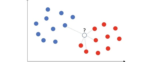
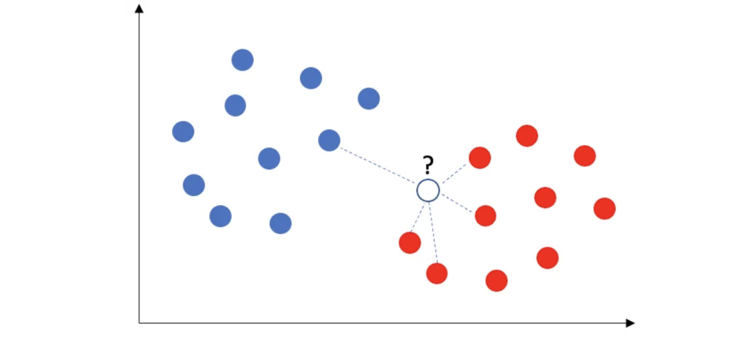
The KNN algorithm is a commonly used supervised learning classification algorithm that predicts the class of new data points based on the assumption that similar data points are usually close to each other. By calculating the distance between the new data point and other data points and selecting the nearest 5 neighbors, the algorithm performs class statistics and then uses a majority voting rule to determine the class. For example, when a new data point appears, if there are 4 neighbors of the red class and 1 neighbor of the blue class, then the new data point will be assigned to the red class.

This process can be summarized as follows: in addition to steps 1 to 3, supervised learning KNN also includes steps 4 and 5:
-
Step 4: Count the number of classes among these K neighbors. -
Step 5: Assign the new data point to the majority class.
How to Define Anomaly Scores?
An outlier is a point that is far away from its neighboring points, and its anomaly score is defined as the distance to its k-th nearest neighbor. Each point has an anomaly score. Our goal is to identify points with high anomaly scores.
The KNN method in PyOD uses one of three distance metrics as the anomaly score: maximum (default), average, and median. The maximum uses the maximum distance to k neighbors as the anomaly score, while the average and median use the average and median as the outlier score, respectively.
Modeling Steps
During the modeling process, step 1 is to build the model and identify outliers. Step 2 involves selecting a threshold to separate outliers from normal observations. In step 3, descriptive statistics of each group are used to analyze both groups to ensure model validity. If the average of a feature in the outlier group does not match expectations, it is necessary to investigate, modify, or discard that feature, and repeat the above steps until expectations are met.
Step 1: Build the Model
Use PyOD’s generate_data() utility to generate data with outliers, containing 10% outliers. It is important to note that although this simulated dataset contains the target variable Y, the unsupervised KNN model only uses the X variables, while the Y variable is only used for validation.
import numpy as np
import pandas as pd
import matplotlib.pyplot as plt
from pyod.utils.data import generate_data
contamination = 0.05 # percentage of outliers
n_train = 500       # number of training points
n_test = 500        # number of testing points
n_features = 6      # number of features
X_train, X_test, y_train, y_test = generate_data(
    n_train=n_train,
    n_test=n_test,
    n_features= n_features,
    contamination=contamination,
    random_state=123)

# Make the 2d numpy array a pandas dataframe for each manipulation
X_train_pd = pd.DataFrame(X_train)

# Plot
plt.scatter(X_train_pd[0], X_train_pd[1], c=y_train, alpha=0.8)
plt.title('Scatter plot')
plt.xlabel('x0')
plt.ylabel('x1')
plt.show()
The yellow points in the scatter plot are the ten percent outliers. The purple points are “normal” observations.
The following code calculates the k-NN model and stores it as knn. Note that there is no y in the function .fit(); in unsupervised methods, y is ignored. def fit(self, X,y=None) If y is specified, it becomes a supervised method.
The next code will build the model and score the training and testing data. The meaning of each line is as follows:
-
label_: The label vector for the training data, which is also used when using.predict()on the training data. -
decision_scores_: The score vector for the training data, which is also used when using.decision_functions()on the training data. -
Decision_score(): The scoring function that assigns anomaly scores to each observation. -
predict(): The prediction function that assigns 1 or 0 based on the specified threshold. -
contamination: The percentage of outliers; PyOD defaults the contamination rate to 10%. This parameter does not affect the calculation of anomaly scores.
from pyod.models.knn import KNN
knn = KNN(contamination=0.05)
knn.fit(X_train)

# Training data
y_train_scores = knn.decision_function(X_train)
y_train_pred = knn.predict(X_train)

# Test data
y_test_scores = knn.decision_function(X_test)
y_test_pred = knn.predict(X_test) # outlier labels (0 or 1)

def count_stat(vector):
    # Because it is '0' and '1', we can run a count statistic.
    unique, counts = np.unique(vector, return_counts=True)
    return dict(zip(unique, counts))

print("The training data:", count_stat(y_train_pred))
print("The training data:", count_stat(y_test_pred))
# Threshold for the defined contamination rate
print("The threshold for the defined contamination rate:" , knn.threshold_)
The training data: {0: 475, 1: 25}
The training data: {0: 475, 1: 25}
The threshold for the defined contamination rate:
0.7566127656515499
Let’s use .get_params() to view the default parameters of KNN. The number of neighbors is 5.0. The contamination rate is set to 5%.
knn.get_params()
{'algorithm': 'auto',
 'contamination': 0.05,
 'leaf_size': 30,
 'method': 'largest',
 'metric': 'minkowski',
 'metric_params': None,
 'n_jobs': 1,
 'n_neighbors': 5,
 'p': 2,
 'radius': 1.0}
Step 2: Determine a Reasonable Threshold
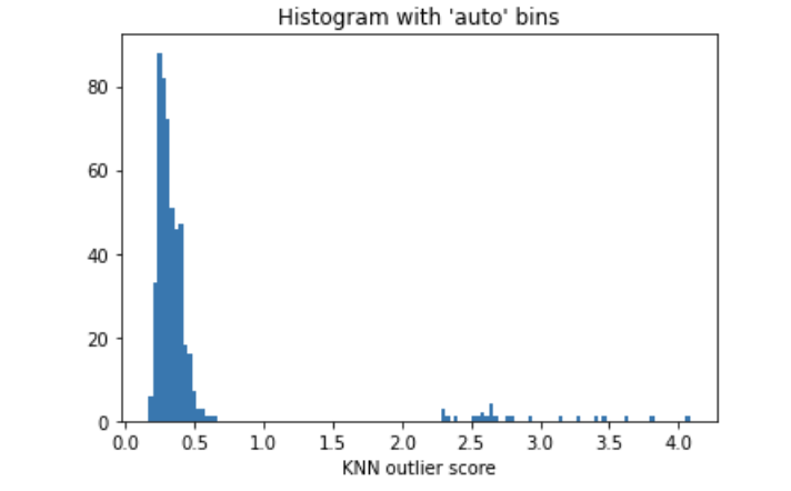
In most cases, we cannot determine the percentage of outliers. We can use the histogram of anomaly scores to select a reasonable threshold. If there is prior knowledge indicating that outliers account for 1%, then a threshold should be selected that results in approximately 1% outliers. The histogram of outlier scores in Figure (D.2) shows a threshold of 200.0, as there is a natural cut point in the histogram. Most data points have low anomaly scores. If we choose 1.0 as the cut point, we can consider those data points >= 1.0 to be outliers.
import matplotlib.pyplot as plt
plt.hist(y_train_scores, bins='auto')  # arguments are passed to np.histogram
plt.title("Histogram with 'auto' bins")
plt.xlabel('KNN outlier score')
plt.show()
Step 3: Analyze Normal and Outlier Groups
Analyzing the normal and outlier groups is a key step in demonstrating model validity. The feature statistics of the normal and outlier groups should be consistent with domain knowledge. If the average of a feature in the outlier group is contrary to expectations, it is recommended to check, modify, or discard that feature. The modeling process should be repeated until all features are consistent with prior knowledge. Additionally, if the data provides new insights, it is also advisable to validate previous knowledge.
threshold = knn.threshold_ # Or other value from the above histogram

def descriptive_stat_threshold(df,pred_score, threshold):
    # Let's see how many '0's and '1's.
    df = pd.DataFrame(df)
    df['Anomaly_Score'] = pred_score
    df['Group'] = np.where(df['Anomaly_Score']< threshold, 'Normal', 'Outlier')

    # Now let's show the summary statistics:
    cnt = df.groupby('Group')['Anomaly_Score'].count().reset_index().rename(columns={'Anomaly_Score':'Count'})
    cnt['Count %'] = (cnt['Count'] / cnt['Count'].sum()) * 100 # The count and count %
    stat = df.groupby('Group').mean().round(2).reset_index() # The avg.
    stat = cnt.merge(stat, left_on='Group',right_on='Group') # Put the count and the avg. together
    return (stat)

descriptive_stat_threshold(X_train,y_train_scores, threshold)
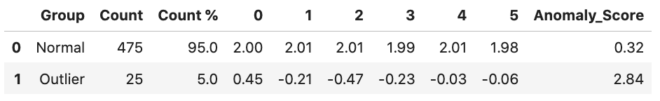
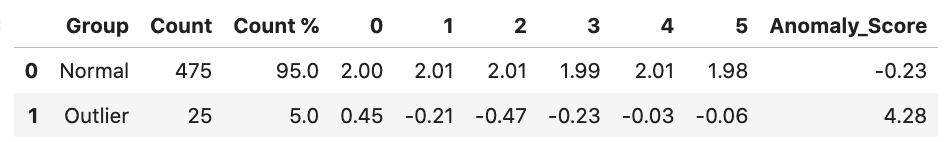
The features of the normal and outlier groups are shown in the table above, including counts and count percentages. The table reveals several key findings:
-
Size of the outlier group: Once the threshold is determined, the size is also determined. The size statistics serve as a good reference, especially when the threshold comes from Figure (D.2) and there is no prior knowledge. -
Feature statistics in each group: All means must be consistent with domain knowledge. In our case, the mean of the outlier group is less than the mean of the normal group. -
Average anomaly score: The average score of the outlier group should be higher than that of the normal group. There is not much explanation needed for the scores.
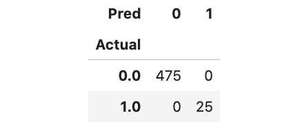
Since we have grasped the basic facts, we can generate a confusion matrix to understand the performance of the model. The model performs excellently, successfully identifying all 25 outliers.
Actual_pred = pd.DataFrame({'Actual': y_test, 'Anomaly_Score': y_test_scores})
Actual_pred['Pred'] = np.where(Actual_pred['Anomaly_Score']< threshold,0,1)
pd.crosstab(Actual_pred['Actual'],Actual_pred['Pred'])
Achieving Model Stability through the Aggregation of Multiple Models
To generate a model with stable results, the best practice is to build multiple KNN models and then aggregate the scores. This approach can reduce the chances of overfitting and improve prediction accuracy.
The PyOD module provides four methods for aggregating results. Only one method is needed to obtain the aggregated results.
-
Average (AVG) -
Maximum of Maximum (MOM) -
Average of Maximum (AOM) -
Maximum of Average (MOA)
I will create 20 KNN models, with k neighbors ranging from 10 to 200.
from pyod.models.combination import aom, moa, average, maximization
from pyod.utils.utility import standardizer
# Standardize data
X_train_norm, X_test_norm = standardizer(X_train, X_test)
# Test a range of k-neighbors from 10 to 200. There will be 20 k-NN models.
k_list = [10, 20, 30, 40, 50, 60, 70, 80, 90, 100, 110,
 120, 130, 140, 150, 160, 170, 180, 190, 200]
n_clf = len(k_list)
# Just prepare data frames so we can store the model results
train_scores = np.zeros([X_train.shape[0], n_clf])
test_scores = np.zeros([X_test.shape[0], n_clf])
train_scores.shape
# Modeling
for i in range(n_clf):
    k = k_list[i]
    clf = KNN(n_neighbors=k, method='largest')
    clf.fit(X_train_norm)

    # Store the results in each column:
    train_scores[:, i] = clf.decision_scores_
    test_scores[:, i] = clf.decision_function(X_test_norm)
# Decision scores have to be normalized before combination
train_scores_norm, test_scores_norm = standardizer(train_scores,test_scores)
# Combination by average
# The test_scores_norm is 500 x 10. The "average" function will take the average of the 10 columns.
# The result "y_by_average" is a single column:
y_train_by_average = average(train_scores_norm)
y_test_by_average = average(test_scores_norm)
import matplotlib.pyplot as plt
plt.hist(y_train_by_average, bins='auto') # arguments are passed to np.histogram
plt.title("Combination by average")
plt.show()
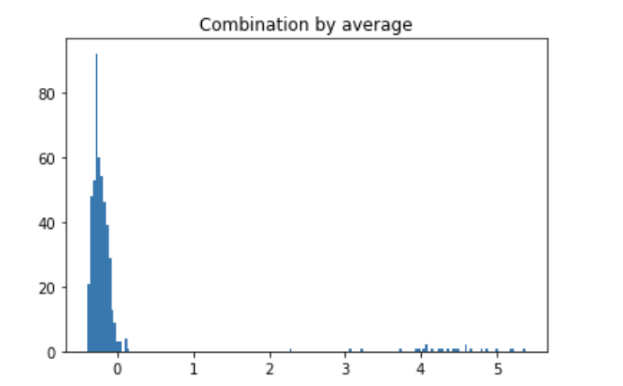
Most data points are below 0.0, with some outliers around 1.0. Setting the threshold to 1.0 or even 2.0 may be more reasonable. This way, an analysis can be performed on the normal and outlier groups. 25 data points were identified as outliers. The mean features of the outlier group are all less than those of the normal group, consistent with the results in the table below.
descriptive_stat_threshold(X_train,y_train_by_average, 0.5)
KNN Algorithm Summary
The unsupervised KNN method uses Euclidean distance to compute the relationships between observations, calculating the distances between neighbors without the need for parameter tuning. KNN defines outliers as the distance to the k-th nearest neighbor.
Recommended Reading