 Python Tribe (python.freelycode.com) organized the translation, welcome to forward, prohibited from reprinting
The k-Nearest Neighbors algorithm (KNN) is based on a simple logic that is easy to understand and implement, making it a powerful tool you can use.
By learning this tutorial, you will be able to implement a KNN algorithm from scratch in Python. This implementation is primarily used to handle classification problems, and we will use the Iris flower classification problem to demonstrate this example.
The requirement for this tutorial is that you should be able to code in Python and be interested in implementing a KNN algorithm.

What is k-Nearest Neighbors?
The KNN model consists of the entire training dataset. When we need to predict an attribute A of a new instance, the KNN algorithm searches the training dataset to find the K most similar instances. The attributes A of these similar instances are summarized to predict the attribute A of the new instance.
How to determine the similarity between instances depends on the type of data. For continuous data, we can use Euclidean distance. For categorical or binary data, we can use Hamming distance.
For regression problems, we can use the average of the predicted values. For classification problems, we can return the most common class.
How does the KNN algorithm work?
The KNN algorithm belongs to instance-based, competitive learning, and lazy learning algorithms.
Instance-based algorithms use data instances (or data rows) to make predictions based on those instances. KNN is an extreme example of instance-based algorithms because all training data become part of the algorithm model.
It is a competitive learning logic because it uses competition among model elements (data instances) to make predictions. The similarity calculations between data instances result in each data instance competing to ‘win’, or compete to be similar to the element that needs to be predicted, or compete to contribute to the prediction results.
It is called a lazy learning algorithm because it only builds a prediction model when a prediction operation is needed; it only starts working when it needs to produce a result.
Its advantage is that only data instances similar to the element that needs to be predicted will play a role; it can be called a local model. The disadvantage is that the computational cost is high because it repeatedly performs similar searches on a large training set.
Finally, KNN is useful because it makes no assumptions about the data while using consistent rules to calculate distances between any two data instances. Because of this, it is called a non-parametric or non-linear algorithm because it does not assume a model function.
Using Measurements to Classify Flowers
The exercise problem used in this tutorial is the classification of Iris flowers.
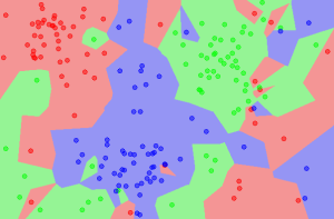
The existing dataset consists of 150 observations of three different species of Iris flowers. There are four measurement dimensions for these flowers: sepal length, sepal width, petal length, and petal width, all measured in centimeters. The attribute to be predicted is the species, which can take the values: Setosa, Versicolor, and Virginica.
We have a standard dataset where the species is known. We can split this dataset into a training dataset and a testing dataset, and then use the testing results to evaluate the accuracy of the algorithm. For this problem, a good classification algorithm should have an accuracy greater than 90%, typically achieving 96% or higher.
You can download this dataset for free from https://archive.ics.uci.edu/ml/machine-learning-databases/iris/iris.data, with more information in the resources section.
How to Implement KNN in Python
This tutorial divides the implementation steps into the following six parts.
-
Data Processing: Read data from CSV and split it into training and testing datasets.
-
Similarity: Calculate the distance between two data instances.
-
Neighbors: Determine the N closest instances.
-
Results: Generate prediction results from these instances.
-
Accuracy: Summarize the accuracy of the predictions.
-
Main Program: String these together.
1. Data Processing
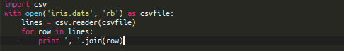
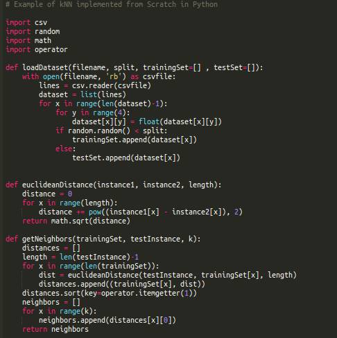
The first thing we need to do is load our data file. The data file is in CSV format and does not have a header row or remarks. We can use the open method to open the file and read the data using the csv module:
 Next, we need to split the dataset into a training dataset for predictions and a testing dataset for accuracy evaluation.
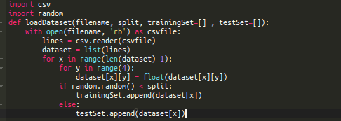
First, we need to convert the loaded feature data from strings to integers. Then we randomly split the training and testing datasets. A common practice is to use a 67/33 ratio for the training/testing data.
Putting this logic together, we get the following function loadDataset:
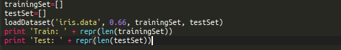
 After downloading the Iris CSV data file to the local folder, we can test our function with the following code:
2. Similarity
To make predictions, we need to calculate the similarity between two data instances. With the similarity calculation function, we can later obtain the N most similar instances to make predictions.
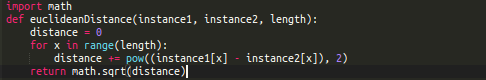
Since the data for the four measurement dimensions of the flowers is numeric and has the same units, we can directly use Euclidean distance for measurement. Euclidean distance is the square root of the sum of the squared differences between corresponding numbers in two columns (similar to the distance formula in a two-dimensional plane, extended to multiple dimensions).
Additionally, we need to determine which dimensions are involved in the calculation. In this problem, we only need to include the four measured dimensions, which are placed in the front of the array. One way to limit dimensions is to add a parameter that tells the function which dimensions to process, ignoring the later dimensions.
Putting this logic together, we get the function to calculate Euclidean distance:
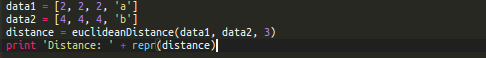
 We can test this function with some dummy data like this:
3. Nearest Elements
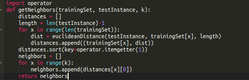
Now that we have a method for calculating similarity, we can get the N data instances closest to the data that needs to be predicted.
The most straightforward way is to calculate the distance from the data to be predicted to all data instances and take the N with the smallest distances.
This logic can be represented by the following function:
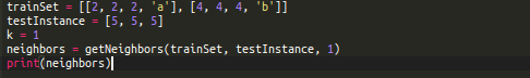
 We can test this function like this:
4. Results
The next task is to obtain prediction results based on the nearest instances.
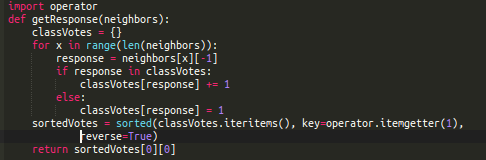
We can have these neighbors vote on the predicted attribute, with the option receiving the most votes being the prediction result.
The following function implements the voting logic, assuming the attribute to be predicted is at the end of the data instance (array).
 We can test it with some test data:
 If the voting result is a tie, this function still returns a prediction result. However, you can handle it your own way, such as returning None in case of a tie or randomly selecting a result.
5. Accuracy
The prediction part has been completed, and now we will evaluate the accuracy of the algorithm.
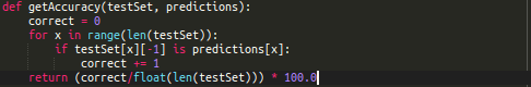
A simple evaluation method is to calculate the proportion of correct predictions made by the algorithm in the testing dataset; this proportion is called classification accuracy.
The following function can calculate classification accuracy.
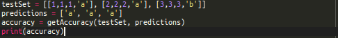
 We can test it with the following example:
6. Main Program
Now that we have all the functions needed for this algorithm, all that’s left is to string them together.
Here is the complete code:
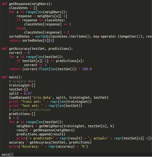 When you run this program, you will see a comparison between each predicted data and the actual data. At the end of the program, you can see the accuracy of this prediction model. In this example, the accuracy is slightly above 98%.
Ideas for Extensions
This section discusses some ideas for extending the Python code provided in this tutorial.
-
Regression: You can adjust the code to allow this algorithm to handle some regression problems (predicting a continuous attribute). For example, when summarizing the nearest instances, use the average or median of the predicted attributes.
-
Normalization: When the units of different attributes vary, some attributes may gain significant weight in determining distances. For such problems, you may need to scale the values of each attribute to between 0-1 before calculation (this process is called normalization). You can improve this algorithm to support data normalization.
-
Replaceable Distance Calculation Methods: There are actually many other distance calculation methods, and you can even develop your own distance calculation method. Implement a replacement distance calculation method, such as Manhattan distance or vector dot product.
You can explore more extension logic, such as giving different weights to instances at different distances during voting, or using a tree structure for searching the nearest instances.
Original English text:http://machinelearningmastery.com/tutorial-to-implement-k-nearest-neighbors-in-python-from-scratch/
Translator: Shishu Sawei
 To learn about wild dogs, please click to read the original text.