Author: Wei Wei

Source:Python Enthusiasts Community

This article contains a total of 7800 words, and it is recommended to read for 10+ minutes.

This article combines code examples to help you get started with Python data mining and machine learning techniques.

This article includes five knowledge points:

1. Introduction to data mining and machine learning techniques

2. Practical Python data preprocessing

3. Introduction to common classification algorithms

4. Practical case study of classifying iris flowers

5. Thought process and techniques for selecting classification algorithms

1. Introduction to Data Mining and Machine Learning Techniques

What is data mining? Data mining refers to the process of processing and analyzing existing data to ultimately obtain deeper relationships between the data. For example, when arranging products in a supermarket, is it more effective to place milk next to bread or next to other products? Data mining techniques can be used to solve such problems. Specifically, the supermarket product placement issue can be categorized under association analysis.

In daily life, data mining techniques are widely applied. For instance, merchants often need to categorize their customers (e.g., SVIP, VIP, regular customers). In this case, a portion of customer data can be used as training data, while another portion can be used as testing data. The training data is then input into a model for training, and after training is complete, the other portion of data is used for testing, ultimately achieving automatic classification of customer levels. Other similar application examples include CAPTCHA recognition, automatic fruit quality screening, etc.

So what is machine learning technology? In short, any technology that allows machines to learn relationships or rules between data through models and algorithms we establish, and ultimately utilize those for our benefit, is considered machine learning technology. In fact, machine learning is an interdisciplinary field that can be roughly divided into two categories: traditional machine learning techniques and deep learning techniques, with deep learning encompassing neural network-related technologies. This course will focus on traditional machine learning techniques and various algorithms.

Since both machine learning and data mining are about exploring the patterns between data, people often mention them together. These two technologies also have a wide range of application scenarios in real life, as illustrated in the following figure:

1. Classification: Classifying customer levels, CAPTCHA recognition, automatic fruit quality screening, etc.

Machine learning and data mining techniques can be used to solve classification problems, such as classifying customer levels, CAPTCHA recognition, and automatic fruit quality screening.

For example, in CAPTCHA recognition, a solution needs to be designed to recognize handwritten digits from 0 to 9. One approach is to first categorize some of the handwritten digits into a training set, then manually map these handwritten digits to their corresponding numerical categories. Once these mappings are established, a classification algorithm can be used to build a corresponding model. If a new handwritten digit appears, this model can predict which numerical category it belongs to. For example, if the model predicts that a handwritten digit belongs to the category of number 1, it can automatically recognize that digit as 1. Therefore, CAPTCHA recognition is essentially a classification problem.

The automatic fruit quality screening problem is also a classification problem. Features such as size and color of the fruit can be mapped to corresponding sweetness categories, for instance, category 1 can represent sweet, while category 0 represents not sweet. After obtaining some training data, a classification algorithm can also be used to build a model. If a new fruit appears, its size and color can automatically determine whether it is sweet or not. This achieves automatic fruit quality screening.

2. Regression: Predicting continuous data, trend forecasting, etc.

In addition to classification, data mining and machine learning techniques also have a classic scenario—regression. In the previously mentioned classification scenarios, the number of categories is limited. For example, in the numerical CAPTCHA recognition scenario, there are digit categories from 0 to 9; similarly, in the letter CAPTCHA recognition scenario, there are limited categories from a to z. Whether digit or letter categories, the number of categories is finite.

Now, assume there exists some data such that after mapping, the best results do not fall on a specific point such as 0, 1, or 2, but rather continuously fall between 1.2, 1.3, 1.4, etc. In this case, classification algorithms cannot solve such problems, and regression analysis algorithms can be used instead. In practical applications, regression analysis algorithms can predict continuous data and trends.

3. Clustering: Customer value prediction, business district prediction, etc.

What is clustering? As mentioned above, to solve classification problems, historical data (i.e., correctly established training data) is necessary. If there is no historical data and one needs to directly categorize an object’s features into their corresponding categories, classification and regression algorithms cannot solve this problem. In such cases, clustering provides a solution. Clustering methods directly categorize objects based on their features without requiring training, making it an unsupervised learning method.

When can clustering be used? For instance, if there is a group of customer feature data in a database, and one needs to categorize these customers into levels (e.g., SVIP customers, VIP customers), clustering models can be used to solve this. Additionally, clustering algorithms can also be used in predicting business districts.

4. Association Analysis: Supermarket product placement, personalized recommendation, etc.

Association analysis refers to analyzing the relationships between items. For example, if a supermarket has a large number of products, one may need to analyze the strength of the association between products, such as between bread and milk. Association analysis algorithms can be used to analyze these relationships directly using user purchase records and other information. Once the associations are understood, they can be applied to supermarket product placement. By placing highly associated products close together, the supermarket can effectively increase product sales.

Furthermore, association analysis can also be used in personalized recommendation technology. For instance, by analyzing user browsing records, one can analyze the associations between various web pages and push strongly associated pages to users while they browse. For example, if analysis of browsing record data reveals a strong association between webpage A and webpage C, when a user is browsing webpage A, webpage C can be pushed to them, thus achieving personalized recommendations.

5. Natural Language Processing: Text similarity technology, chatbots, etc.

In addition to the aforementioned application scenarios, data mining and machine learning techniques can also be applied to natural language processing and speech processing, such as calculating text similarity and chatbots.

2. Practical Python Data Preprocessing

Before performing data mining and machine learning, the first step is to preprocess the existing data. If the initial data is incorrect, the accuracy of the final results cannot be guaranteed. Only by preprocessing the data to ensure its accuracy can we ensure the correctness of the final results.

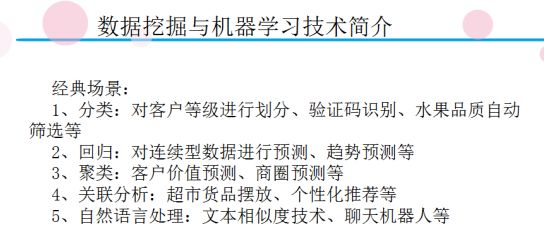
Data preprocessing refers to the initial processing of data to eliminate dirty data (i.e., data that affects result accuracy); otherwise, it can easily influence the final results. Common data preprocessing methods are shown in the following diagram:

1. Handling Missing Values

Missing values refer to the absence of certain feature values in a set of data. There are two methods to address missing values: one is to delete the row of data with the missing value, and the other is to fill the missing value with a correct value.

2. Handling Outliers

Outliers often arise from errors during data collection, such as mistakenly recording 68 as 680. Before addressing outliers, it is necessary to first identify these outlier data, which can often be accomplished using graphical methods. After processing the outlier data, the original data can be brought closer to accuracy, ensuring the correctness of the final results.

3. Data Integration

Compared to handling missing values and outliers, data integration is a relatively simple method of data preprocessing. So what is data integration? Suppose there are two groups of data, A and B, with the same structure, both of which are loaded into memory. If the user wants to merge these two groups into one, they can directly use Pandas to merge them, which is essentially data integration.

Next, using Taobao product data as an example, we will introduce the practical application of the aforementioned preprocessing steps.

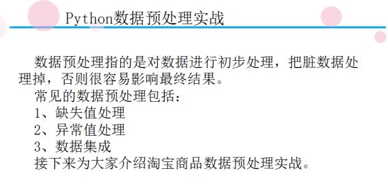
Before data preprocessing, we first need to import Taobao product data from the MySQL database. After starting the MySQL database, we query the taob table and obtain the following output:

It can be seen that the taob table contains four fields. The title field stores the names of Taobao products; the link field stores the links to Taobao products; the price field stores the prices of Taobao products; and the comment field stores the number of comments on Taobao products (which somewhat represents product sales).

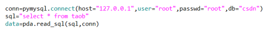
So how do we import this data? First, we connect to the database using pymysql (if there are encoding issues, modify the source code of pymysql). After a successful connection, we retrieve all data from the taob table, and then we can use the read_sql() method in pandas to import the data into memory.

The read_sql() method has two parameters: the first parameter is the SQL statement, and the second parameter is the connection information for the MySQL database. The specific code is shown in the following figure:

1. Handling Missing Values in Practice

Handling missing values can be done through data cleaning. Using the example of Taobao product data, a product’s comment count may be 0, but its price cannot be 0. However, in reality, there are some data with a price of 0 in the database, which occurs because the price attribute of some data was not crawled.

So how can we determine if these data have missing values? This can be done using the following method:

First, call the data.describe() method on the previous taob table, which will yield the following results:

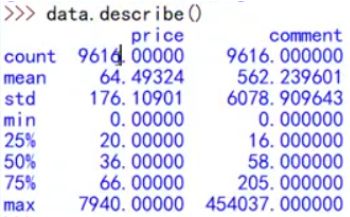
How to interpret these statistical results? The first step is to pay attention to the count data of the price and comment fields. If the counts are not equal, it indicates that there is missing information; if they are equal, it is not immediately clear whether there are missing values. For example, if the count of price is 9616.0000 and the count of comment is 9615.0000, it indicates that at least one comment data is missing.

The meanings of the other fields are as follows: mean represents the average; std represents the standard deviation; min represents the minimum value; max represents the maximum value.

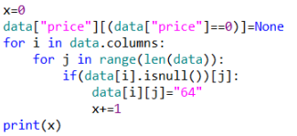
How can we handle these missing data? One method is to delete these data, while another method is to insert a new value in place of the missing value. The value in the second method can be the mean or median, and whether to use the mean or median should be decided based on the actual situation. For example, for age data (ranging from 1 to 100 years), stable data with small variation generally uses the mean, while data with larger variation generally uses the median.

The specific operation to handle missing values for price is as follows:

2. Handling Outliers in Practice

Similar to the process of handling missing values, to handle outliers, we first need to identify them. Outliers are usually discovered through scatter plots, as similar data will cluster in one area of the scatter plot, while outliers will be spread far from that area. Based on this property, it is quite easy to find outlier data. The specific operation is shown in the following figure:

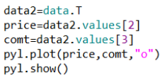
First, we need to extract price and comment data from the dataset. The usual approach may involve looping to extract them, but this method is too complex. A simpler method is to transpose the data frame, turning the original column data into row data, making it easy to access price and comment data. Next, we can use the plot() method to create a scatter plot, where the first parameter represents the x-axis, the second parameter represents the y-axis, and the third parameter specifies the type of plot, with “o” representing a scatter plot. Finally, we can use the show() method to display it, allowing us to visually observe the outliers. These outliers do not help in data analysis, and in practice, we often need to delete or convert the data of these outliers into normal values. The following is the scatter plot created:

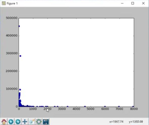
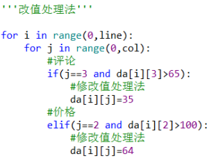
Based on the above figure, we can process the data where comments exceed 100,000 and prices exceed 1,000, achieving the effect of handling outliers. The specific implementation process for the two processing methods is as follows:

The first method is to change the values, replacing them with the median, mean, or other values. The specific operation is shown in the following figure:

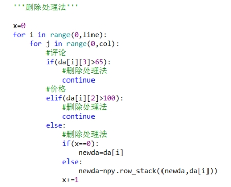
The second method is to delete the outlier data directly, which is also a recommended method. The specific operation is shown in the following figure:

3. Distribution Analysis

Distribution analysis refers to analyzing the distribution state of data, i.e., observing whether it is linearly distributed or normally distributed. This is generally done using histograms. The steps for creating a histogram are as follows: calculate the range, calculate the class interval, and draw the histogram. The specific operation is shown in the following figure:

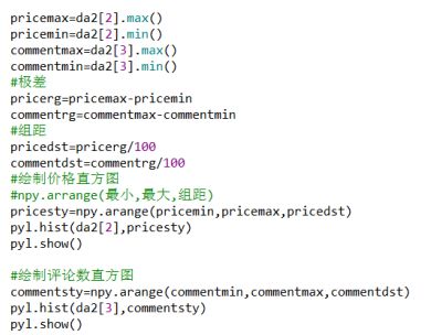
In this case, the arrange() method is used to specify the style, where the first parameter represents the minimum value, the second parameter represents the maximum value, and the third parameter represents the class interval. Next, we use the hist() method to draw the histogram.

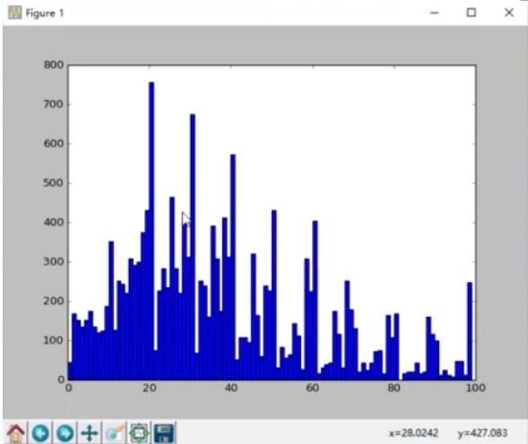
The histogram of Taobao product prices in the taob table is shown in the following figure, which roughly follows a normal distribution:

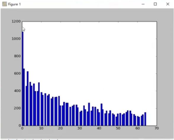
The histogram of comments for Taobao products in the taob table is shown in the following figure, which roughly follows a decreasing curve:

4. Drawing a Word Cloud

Sometimes it is necessary to draw a word cloud based on a piece of text information. The specific operation for drawing is shown in the following figure:

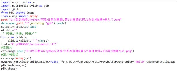
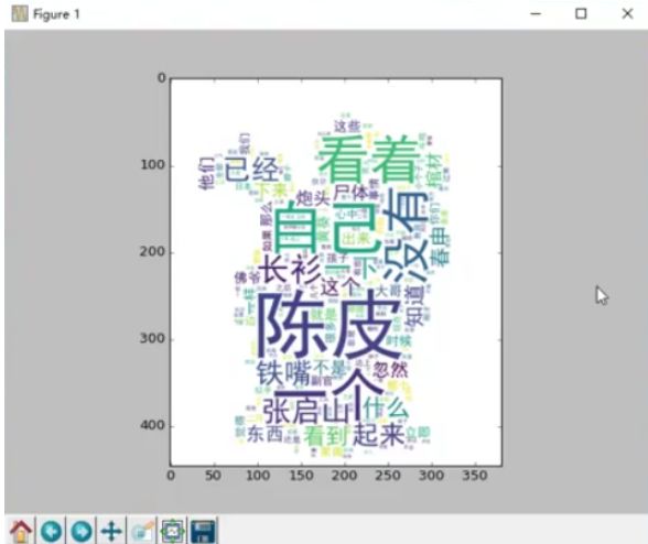
The general process is as follows: first use cut() to segment the document, and after segmentation, organize these words into a fixed format. Then, according to the desired presentation form of the word cloud, read the corresponding image (the word cloud in the following figure is shaped like a cat), and finally use wc.WordCloud() to convert it into a word cloud, displaying it using imshow(). For example, the word cloud drawn based on the document “Old Nine Gates.txt” is shown in the following figure:

3. Introduction to Common Classification Algorithms

There are many common classification algorithms, as shown in the following figure:

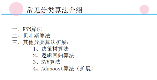
Among them, KNN and Naive Bayes algorithms are quite important, in addition to other algorithms such as decision tree algorithm, logistic regression algorithm, and SVM algorithm. The Adaboost algorithm is mainly used to enhance weak classification algorithms.

4. Practical Case Study of Classifying Iris Flowers

Suppose there are some data on iris flowers, which include features such as petal length, petal width, sepal length, and sepal width. With this historical data, we can train a classification model. Once the model training is complete, when a new unknown type of iris flower appears, we can use the trained model to determine its type. This case can be implemented in various ways, but which classification algorithm would work better?

1. KNN Algorithm

Introduction to KNN Algorithm:

First, consider a problem in the previously mentioned Taobao products, which includes three types of products: snacks, branded bags, and electronics. They have two features: price and comment count. When sorted by price, branded bags are the most expensive, followed by electronics, and snacks are the cheapest; when sorted by comment count, snacks have the most comments, followed by electronics, and branded bags have the least. Then, we can establish a Cartesian coordinate system with price as the x-axis and comment count as the y-axis, plotting the distribution of these three types of products in the coordinate system, as shown in the following figure:

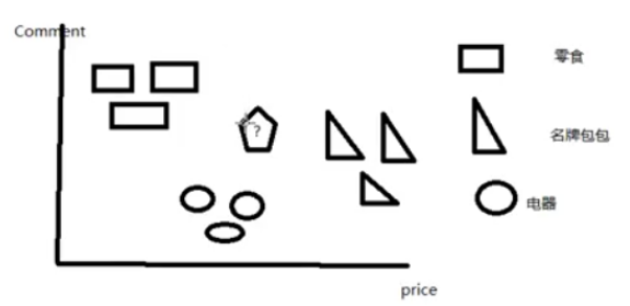
It is clear that these three types of products are concentrated in different areas. If a new product with known features appears, represented by ?, we can determine which of the three types it most likely belongs to based on its features. This type of problem can be solved using the KNN algorithm. The implementation idea is to calculate the sum of the Euclidean distances from the unknown product to each of the other products, then sort them. The smaller the sum of distances, the more similar the unknown product is to that type. For example, if after calculations the Euclidean distance sum to the electronics category is the smallest, we can conclude that the product belongs to the electronics category.

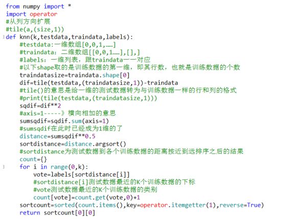
Implementation Method:

The specific implementation of the above process is as follows:

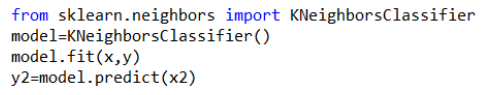
Of course, one can also use a library, which is simpler and more convenient, but the downside is that users may not understand the underlying principles:

Using KNN Algorithm to Solve the Classification Problem of Iris Flowers:

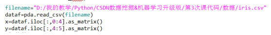
First, load the iris flower data. There are two ways to load it: one is to read directly from the iris dataset; after setting the path, use the read_csv() method to read it, separating the features and results of the dataset, as shown in the following operation:

Another loading method is to use sklearn to implement loading. The datasets in sklearn include the iris dataset, which can be loaded using the datasets.load_iris() method. Subsequently, we can also obtain features and categories, and then separate training and testing data (usually for cross-validation) using the train_test_split() method, where the third parameter represents the test proportion, and the fourth parameter is the random seed, as shown in the following operation:

Once loading is complete, we can utilize the KNN algorithm mentioned earlier for classification.

2. Naive Bayes Algorithm

Introduction to Naive Bayes Algorithm:

First, let’s introduce the Naive Bayes formula: P(B|A) = P(A|B)P(B)/P(A). Suppose we have some course data as shown in the table below, where price and class hours are features of the course, and sales are the result of the course. If a new course appears with a high price and many class hours, we can predict its sales based on existing data.

Price (A)	Class Hours (B)	Sales (C)
Low	Many	High
High	Medium	High
Low	Few	High
Low	Medium	Low
Medium	Medium	Medium
High	Many	High
Low	Few	Medium

Clearly, this problem is a classification problem. First, we need to process the table by transforming features one and two into numbers, with 0 representing low, 1 representing medium, and 2 representing high. After digitization, [[t1,t2],[t1,t2],[t1,t2]]——[[0,2],[2,1],[0,0]] is obtained, then transposing this two-dimensional list (to facilitate subsequent statistics) yields [[t1,t1,t1],[t2,t2,t2]]——-[[0,2,0],[2,1,0]]. Here, [0,2,0] represents the prices of various courses, while [2,1,0] represents the class hours of various courses.

The original problem can be equated to finding the probabilities of the new course’s sales being high, medium, or low given the conditions of high price and many class hours. In other words, we need to compare P(c0|AB), P(c1|AB), and P(c2|AB) for three scenarios, where C has three cases: c0=high, c1=medium, c2=low. The calculations are as follows:

P(c0|AB)=P(A|C0)P(B|C0)P(C0)=2/4*2/4*4/7=1/7

P(c1|AB)=P(A|C1)P(B|C1)P(C1)=0=0

P(c2|AB)=P(A|C2)P(B|C2)P(C2)=0=0

Clearly, P(c0|AB) is the largest, indicating that the predicted sales for the new course is high.

Implementation Method:

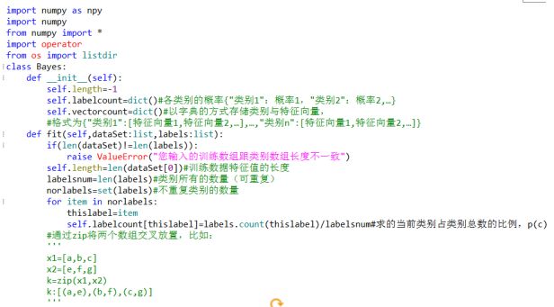
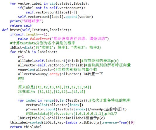
Similar to the KNN algorithm, the Naive Bayes algorithm can also be implemented in two ways: one is a detailed implementation:

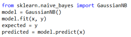
The second method is an integrated implementation:

3. Decision Tree Algorithm

The decision tree algorithm is implemented based on the theory of information entropy. The calculation process of this algorithm is divided into the following steps:

• First, calculate the total information entropy

• Calculate the information entropy of each feature

• Calculate E and information gain, where E = total information entropy – information gain, and information gain = total information entropy – E

• If E is smaller, the information gain is larger, and the uncertainty factor is smaller

A decision tree is formed by considering whether to include each feature for multi-featured data (0 for not considering, 1 for considering), eventually forming a binary tree after considering all features. The following figure illustrates a decision tree:

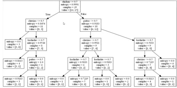
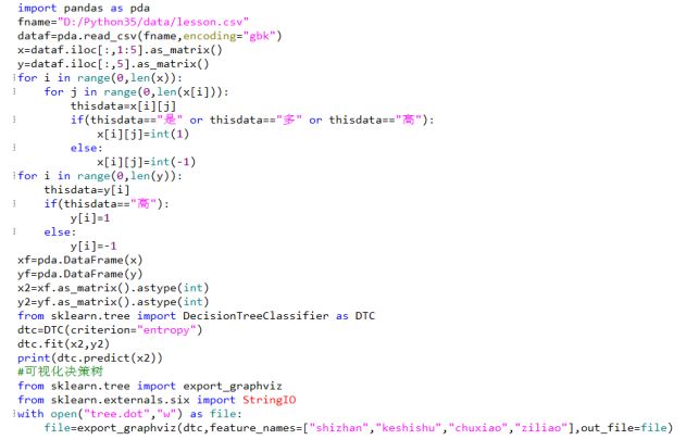
The implementation process of the decision tree algorithm involves first extracting the categories of data, then transforming the data into a descriptive format (for example, converting “yes” to 1 and “no” to 0), using sklearn’s DecisionTreeClassifier to build the decision tree, training the data with the fit() method, and finally using export_graphviz for visualization of the decision tree. The specific implementation process is shown in the following figure:

4. Logistic Regression Algorithm

The logistic regression algorithm is implemented using the principles of linear regression. Suppose there exists a linear regression function: y = a1x1 + a2x2 + a3x3 + … + anxn + b, where x1 to xn represent various features. Although this line can fit the data, the range of y is too large, resulting in poor robustness. To achieve classification, we need to reduce the range of y to a certain space, such as [0,1]. This can be achieved through a change of variable:

Let y = ln(p/(1-p))

Then: e^y = e^(ln(p/(1-p)))

=> e^y = p/(1-p)

=> e^y * (1-p) = p => e^y – p * e^y = p

=> e^y = p(1 + e^y)

=> p = e^y/(1 + e^y)

=> p belongs to [0,1]

This reduces the range of y, allowing for precise classification, thus achieving logistic regression.

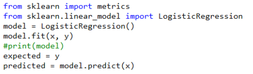
The implementation process of the logistic regression algorithm is shown in the following figure:

5. SVM Algorithm

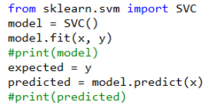
The SVM algorithm is a precise classification algorithm, but its interpretability is not strong. It can transform problems that are linearly inseparable in low-dimensional space into linearly separable problems in high-dimensional space. The SVM algorithm is very simple to use: just import SVC, train the model, and make predictions. The specific operation is shown in the following figure:

Although the implementation is very simple, the key to this algorithm lies in how to choose the kernel function. Kernel functions can be divided into several types, each suitable for different situations:

• Linear Kernel Function

• Polynomial Kernel Function

• Radial Basis Kernel Function

• Sigmoid Kernel Function

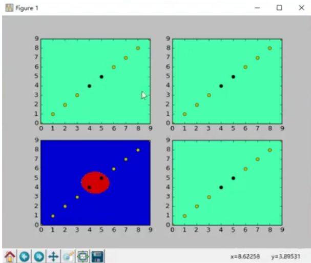
For data that is not particularly complex, one can use linear or polynomial kernel functions. For complex data, the radial basis kernel function is preferred. The images produced by different kernel functions are shown in the following figure:

5. Adaboost Algorithm

Suppose there is a single-layer decision tree algorithm, which is a weak classification algorithm (with low accuracy). If we want to strengthen this weak classifier, we can implement it using the boosting idea, such as using the Adaboost algorithm, which involves multiple iterations, assigning different weights each time, while calculating error rates and adjusting weights, ultimately forming a comprehensive result.

The Adaboost algorithm is generally not used alone but is combined with other algorithms to enhance weak classification algorithms.

5. Thought Process and Techniques for Selecting Classification Algorithms

First, determine whether it is a binary classification or multi-class classification problem. If it is a binary classification problem, generally any of these algorithms can be used; if it is a multi-class classification problem, KNN and Naive Bayes algorithms can be used. Next, consider whether high interpretability is required; if so, SVM cannot be used. Also, consider the number of training samples; if the number of training samples is too large, KNN is not suitable. Finally, consider whether weak-strong algorithm transformation is needed; if so, use the Adaboost algorithm; otherwise, do not. If uncertain, one can select a portion of data for validation and evaluate the model (in terms of time consumption and accuracy).

In summary, the advantages and disadvantages of various classification algorithms can be summarized as follows:

KNN: Multi-class, lazy evaluation, not suitable for large training data

Naive Bayes: Multi-class, large computational load, features cannot be correlated

Decision Tree Algorithm: Binary classification, very good interpretability

Logistic Regression Algorithm: Binary classification, no need for features to be correlated

SVM Algorithm: Binary classification, performs well but lacks interpretability

Adaboost Algorithm: Suitable for strengthening weak classification algorithms