In fact, artificial intelligence has been part of our lives for a long time. However, for many people, artificial intelligence is still a relatively “profound” technology,but no matter how profound the technology is, it starts from basic principles.. There are ten major algorithms in the field of artificial intelligence, which are simple in principle, discovered and applied a long time ago, and you may have learned them in high school, being very common in life.
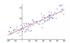
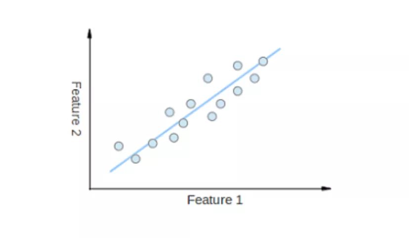
Linear Regression (Linear Regression) is probably the most popular machine learning algorithm. Linear regression aims to find a line that fits the data points in a scatter plot as closely as possible. It attempts to represent the independent variable (x value) and the numerical outcome (y value) by fitting the line equation to the data. This line can then be used to predict future values!
The most commonly used technique for this algorithm is Least Squares. This method calculates the best fit line to minimize the vertical distance from each data point to the line. The total distance is the sum of the squares of the vertical distances (green line) from all data points. The idea is to fit the model by minimizing this squared error or distance.
For example, in simple linear regression, it has one independent variable (x-axis) and one dependent variable (y-axis).
For instance, predicting next year’s housing price increase, or the sales of a new product in the next quarter, etc. It doesn’t sound difficult, but the challenge of the linear regression algorithm lies not in obtaining the predicted value, but in how to be more precise. For that possibly very subtle number, how many engineers have exhausted their youth and hair.
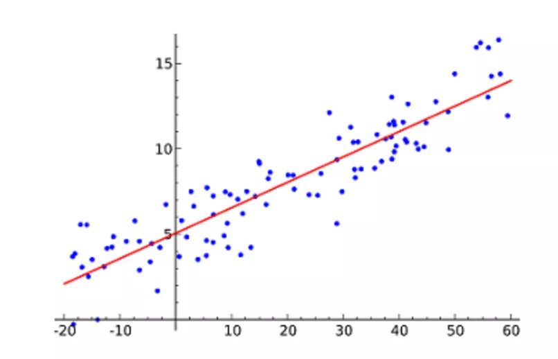
Logistic Regression (Logistic Regression) is similar to linear regression, but the result of logistic regression can only have two values. While linear regression predicts an open numerical value, logistic regression is more like a true or false question.
The range of Y values in the logistic function is from 0 to 1, which is a probability value. The logistic function typically has an S-shaped curve, dividing the chart into two regions, making it suitable for classification tasks.
For example, the logistic regression curve above shows the relationship between the probability of passing an exam and study time, which can be used to predict whether one can pass the exam.
Logistic regression is often used by e-commerce or food delivery platforms to predict user purchasing preferences for categories.
If linear and logistic regression complete tasks in one round, thenDecision Trees (Decision Trees) represent a multi-step action, also used in regression and classification tasks, but the scenarios are usually more complex and specific.
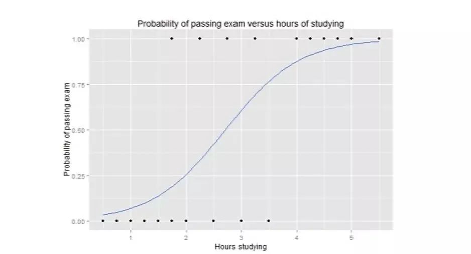
For a simple example, a teacher facing a class of students has to determine who the good students are. If simply judging that a score of 90 is good seems too rough, then we can discuss students with scores below 90 based on homework, attendance, and questioning.
The above is an illustration of a decision tree, where each forked circle is called a node. At each node, we ask questions about the data based on the available features. The left and right branches represent possible answers. The final nodes (i.e., leaf nodes) correspond to a predicted value.
The importance of each feature is determined by a top-down approach. The higher the node, the more important its attribute. For instance, in the above example, the teacher considers attendance more important than homework, so the attendance node is higher, and of course, the score node is higher.
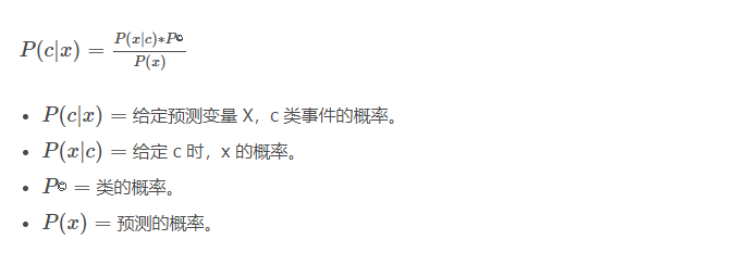
Naive Bayes (Naive Bayes) is based on Bayes’ theorem, which is about the conditional relationship between two conditions. It measures the probability of each class, with the conditional probability of each class given the value of x. This algorithm is used for classification problems, yielding a binary “yes/no” result. Take a look at the equation below.
The Naive Bayes classifier is a popular statistical technique, with a classic application being spam filtering.
Of course, I bet a hot pot that 80% of people did not understand the above statement. (The 80% figure is just my guess, but experiential intuition is a kind of Bayesian calculation.)
To explain Bayes’ theorem in non-technical terms, it is to derive the probability of A given that B occurs, from the probability of B given that A occurs. For instance, if a kitten likes you, there is a % chance it will roll over in front of you; how likely is it that the kitten rolling over in front of you likes you?
Of course, doing questions like this is akin to grasping at straws, so we need to introduce other data, such as the kitten has a % chance of cuddling with you, and a % chance of purring. So how do we know how likely the kitten likes itself? We can calculate it using Bayes’ theorem from the probabilities of rolling over, cuddling, and purring.
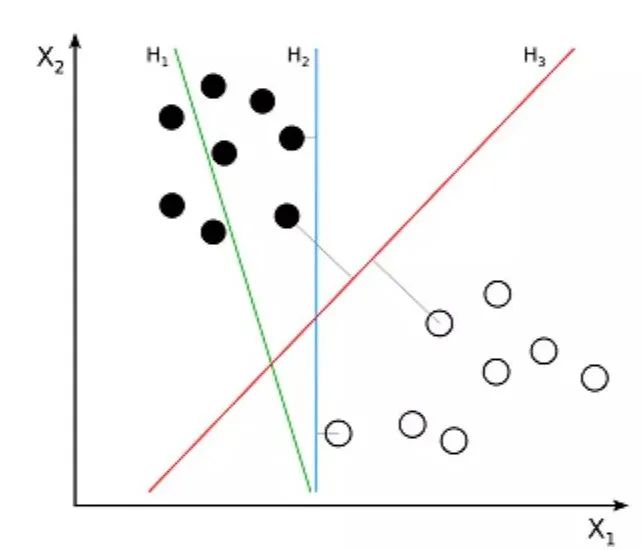
Support Vector Machine (Support Vector Machine, SVM) is a supervised algorithm used for classification problems. The support vector machine tries to draw two lines between data points, maximizing the margin between them. To do this, we plot the data items as points in n-dimensional space, where n is the number of input features. Based on this, the support vector machine finds an optimal boundary, called a hyperplane, which best separates the possible outputs by class labels.
The distance between the hyperplane and the nearest class point is called the margin. The optimal hyperplane has the largest boundary, allowing for classification of points while maximizing the distance between the nearest data points and the two classes.
Thus, the problem that the support vector machine aims to solve is how to distinguish a bunch of data, with its main applications including character recognition, face recognition, text classification, and various other recognitions.
K-Nearest Neighbors (KNN)
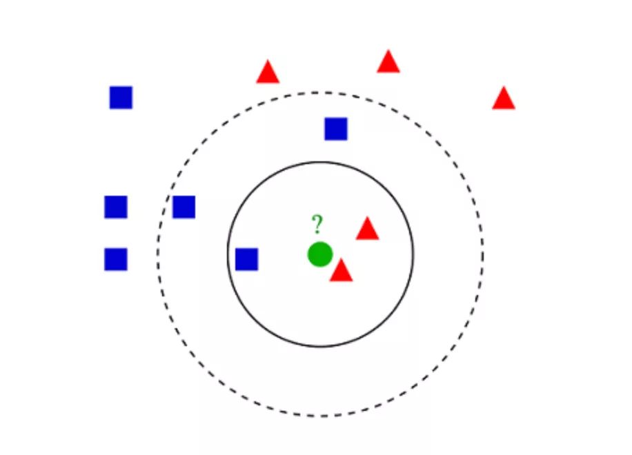
K-Nearest Neighbors (KNN) is very simple. KNN classifies objects by searching the K most similar instances (neighbors) in the entire training set and assigning a common output variable to all these K instances.
The choice of K is crucial: a smaller value may lead to a lot of noise and inaccurate results, while a larger value is unfeasible. It is most commonly used for classification, but can also be applied to regression problems.
The distance used to evaluate the similarity between instances can be Euclidean distance, Manhattan distance, or Minkowski distance. Euclidean distance is the ordinary straight-line distance between two points. It is essentially the square root of the sum of the squares of the differences in point coordinates.
KNN classification example
KNN theory is simple and easy to implement, applicable for text classification, pattern recognition, clustering analysis, etc.
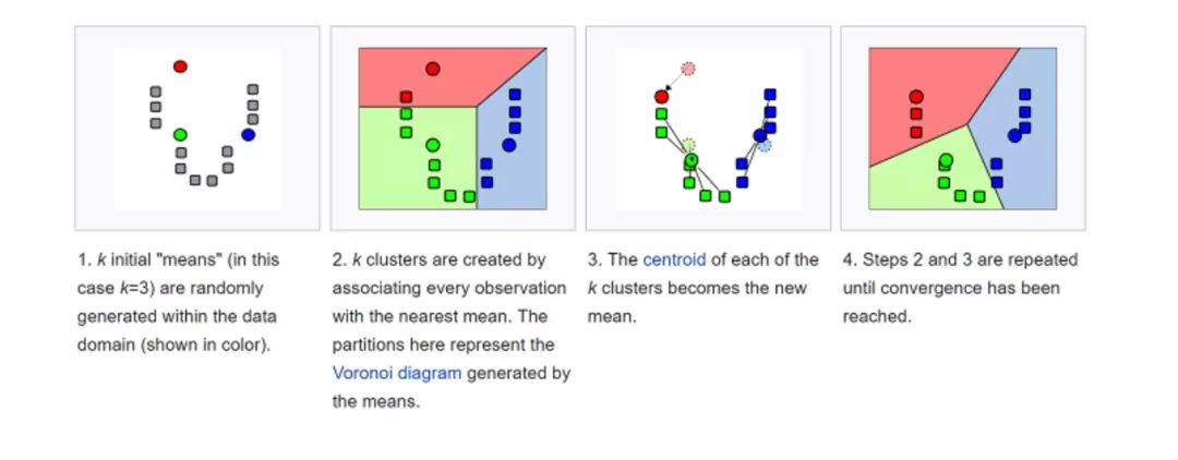
K-means is a clustering algorithm that categorizes data sets. For example, this algorithm can be used to group users based on purchase history. It finds K clusters in the data set. K-means is used in unsupervised learning, so we only need to use the training data X, along with the number of clusters K we want to identify.
The algorithm iteratively assigns each data point to one of the K groups based on the features of each data point. It selects K points as K-cluster centroids. Based on similarity, new data points are added to the cluster with the nearest centroid. This process continues until the centroids stop changing.
In real life, K-means plays an important role in fraud detection, widely used in the fields of automotive, healthcare insurance, and insurance fraud detection.
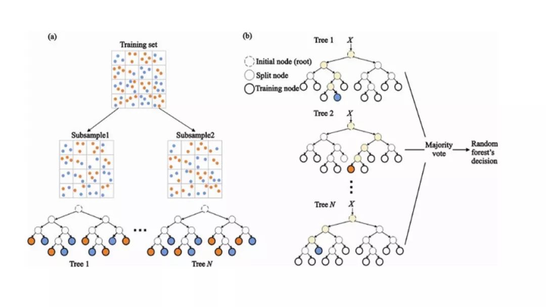
Random Forest (Random Forest) is a very popular ensemble machine learning algorithm. The basic idea of this algorithm is that the opinions of many people are more accurate than those of individuals. In Random Forest, we use an ensemble of decision trees (see Decision Trees).
(a) During training, each decision tree is constructed based on bootstrapped samples from the training set.
(b) During classification, the decision for the input instance is made based on majority voting.
Random Forest has a wide range of application prospects, from marketing to healthcare insurance, it can be used for modeling marketing simulations, statistical customer acquisition, retention, and churn, as well as predicting disease risks and patient susceptibility.
Due to the vast amount of data we can capture today, machine learning problems have become more complex. This means extremely slow training and difficulty in finding a good solution. This issue is often referred to as the “Curse of Dimensionality“.
Dimensionality reduction attempts to solve this problem by combining specific features into higher-level features without losing the most important information. Principal Component Analysis (PCA) is the most popular dimensionality reduction technique.
PCA reduces the dimensionality of the dataset by compressing it into low-dimensional lines or hyperplanes/subspaces, retaining the significant features of the original data as much as possible.
An example of dimensionality reduction can be achieved by approximating all data points to a straight line.
Artificial Neural Networks (ANN)
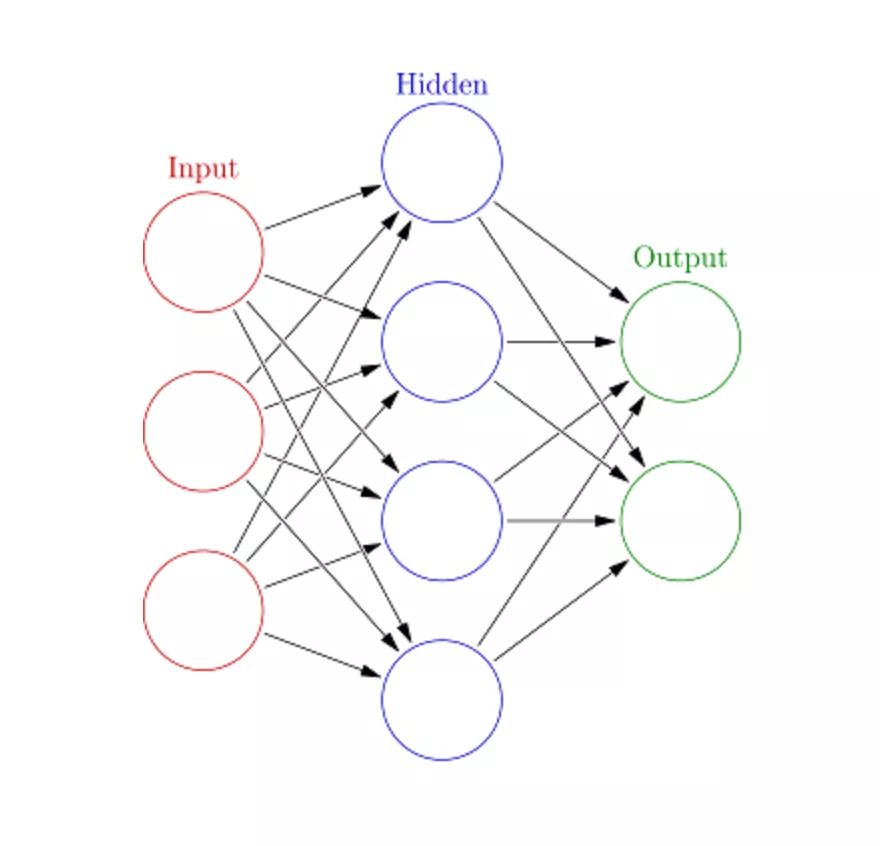
Artificial Neural Networks (ANN) can handle large and complex machine learning tasks. Neural networks are essentially a set of interconnected layers made up of edges and nodes with weights, known as neurons. Between the input layer and the output layer, we can insert multiple hidden layers. Artificial Neural Networks use two hidden layers. Additionally, deep learning needs to be addressed.
The working principle of artificial neural networks resembles the structure of the brain. A set of neurons is assigned a random weight to determine how the neurons process input data. By training the neural network on input data, it learns the relationship between inputs and outputs. During the training phase, the system has access to the correct answers.
If the network cannot accurately recognize the input, the system will adjust the weights. After sufficient training, it will consistently recognize the correct patterns.
Each circular node represents an artificial neuron, and the arrows indicate the connections from the output of one artificial neuron to the input of another.
Image recognition is a well-known application within neural networks.
Now, you have a basic understanding of the most popular artificial intelligence algorithms and some recognition of their practical applications.