Introduction to KNN Algorithm in Machine Learning

CodingGo Technical Community

A Free Programming Learning Platform

Algorithm Introduction

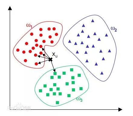
KNN (K-Nearest Neighbors) is a simple machine learning algorithm that does not require learning any parameters and can be used for both classification and regression problems. The intuitive explanation of this algorithm is ‘Birds of a feather flock together.’ When a new sample is input, it estimates the new input sample based on the values of nearby samples. As shown in the figure below, the new input sample will be classified as W1.

Factors Affecting the Algorithm

After understanding the general idea of the algorithm, there are still several questions that need further exploration:

1. How to express the distance (similarity) between two samples?

2. How should the K value in KNN be selected?

3. After determining the neighboring points, how to derive the final result?

Distance Calculation:

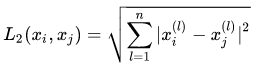
First, we map the features of each sample into feature space. The measurement of sample distance is actually the distance between two points in space, and the Euclidean distance is generally used.

The choice of distance calculation method depends on the specific scenario and the problem to be solved (domain knowledge). For example, when predicting house prices based on latitude and longitude information, the distance can be directly calculated using the latitude and longitude distance formula.

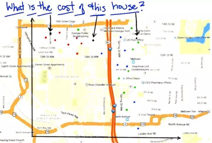
Predicting the house price of the black dot

K Value Selection:

The choice of K value has a significant impact on the final result. If we select a very small K value, the samples can easily be influenced by surrounding outliers, making the model prone to overfitting.

The figure below shows the effect when K is set to 1. It is evident that the boundary is very rough, and some outliers severely affect the classification result.

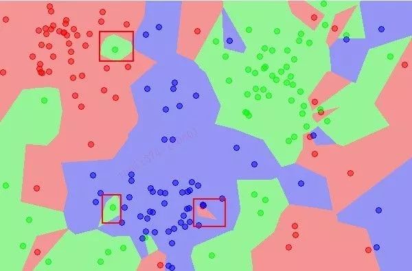Classification effect with K set to 1

If a larger K value is chosen, it is equivalent to using a larger range of training instances for prediction, which can reduce the influence of outlier data. If K is set to the size of the entire sample, the final result is equivalent to averaging the entire sample, making the model too simplistic.

In summary: The smaller the K value, the more prone the model is to overfitting. The larger the value, the simpler the model becomes, making it difficult to detect differences in the data.

Decision Process After Determining Neighboring Points:

Generally, the final prediction result is determined by averaging or majority voting over the K values. Different weights can also be applied to each type or based on the distance, depending on the business scenario.

Algorithm Implementation:

Below is a very simple implementation, which requires traversing the entire sample set each time and finally averaging to obtain the prediction result.

import numpy as np
from sklearn.neighbors import KNeighborsClassifier
from sklearn.metrics.pairwise import pairwise_distances
''' 
# samples are the samples to be classified
# topk is the Number of neighbors
''' 
def predict_by_k_nearest(samples, features, labels, topk):
    distance = [pairwise_distances(i, samples)[0][0] for i in features]
    index = np.argsort(distance)[:topk]
    return 1 if (y[index].mean() > 0.5) else 0

Completing the classification process, we verified it using sklearn’s KNeighborsClassifier and found that the prediction result is always 1. The KNeighborsClassifier from sklearn has different parameters that can be set, all revolving around the three questions we discussed earlier.

X = np.asarray([[0], [1], [2], [3], [4]])
y = np.asarray([0, 0, 1, 1, 1])

neigh = KNeighborsClassifier(n_neighbors=3, weights='uniform')
neigh.fit(X, y)
print(neigh.predict([[3]]))
print (predict_by_k_nearest([3], X, y, 3))
### [1]

Additional:

KNN requires traversing all samples every time to calculate distances, which is very time-consuming. We can use KD trees to optimize the query process. The core idea is to index similar samples in the same range, so that during each query, only nearby ranges need to be examined. I have not implemented this part, but interested students can search for relevant materials online.

▼ Long press to scan the QR code above or click the link below to read the original text and participate

Netease Cloud Classroom launched“Machine Learning Engineer” Micro-professional Course