Introduction to Deep Learning Algorithms for Time Series Forecasting

1 Overview

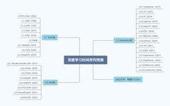
Deep learning methods are a type of machine learning that utilizes neural network models for advanced pattern recognition and automatic feature extraction. In recent years, they have achieved great results in the field of time series forecasting. Commonly used deep learning models include Recurrent Neural Networks (RNN), Long Short-Term Memory networks (LSTM), Gated Recurrent Units (GRU), Convolutional Neural Networks (CNN), Attention mechanisms, and Hybrid models. Compared to traditional machine learning that requires complex feature engineering, these models usually only need data preprocessing, network structure design, and hyperparameter tuning to output time series forecasting results end-to-end.

Deep learning algorithms can automatically learn patterns and trends in time series data. Neural networks involve important parameters such as the number of hidden layers, number of neurons, learning rate, and activation functions. For complex nonlinear patterns, deep learning models have strong expressive capabilities. When applying deep learning methods for time series forecasting, it is necessary to consider the stationarity and periodicity of the data, choose suitable models and parameters, train and test them, and perform model tuning and validation.

2 Algorithm Display

2.1 RNN Class

In RNNs, the input at each moment and the state from the previous moment are mapped to the hidden state. At the same time, based on the current input and previous state, the output for the next moment is predicted. An important feature of RNNs is their ability to handle variable-length sequence data, making them very suitable for time series data in forecasting. Additionally, RNNs can enhance their expressive and memory capabilities by incorporating gating mechanisms such as LSTM, GRU, and SRU.

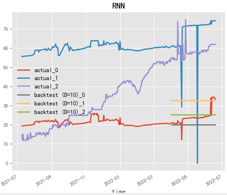
2.1.1 RNN (1990)

Paper: Finding Structure in Time

RNN (Recurrent Neural Network) is a powerful deep learning model frequently used for time series forecasting. RNNs unfold the neural network over time, passing historical information into the future, thus capable of handling the temporal dependencies and dynamic changes in time series data. In constructing RNN models, LSTM and GRU models are often used since they can handle long sequences and have memory cells and gating mechanisms that effectively capture temporal dependencies in time series.

# RNNmodel = RNNModel(    model="RNN",    hidden_dim=60,    dropout=0,    batch_size=100,    n_epochs=200,    optimizer_kwargs={"lr": 1e-3},    # model_name="Air_RNN",    log_tensorboard=True,    random_state=42,    training_length=20,    input_chunk_length=60,    # force_reset=True,    # save_checkpoints=True,)

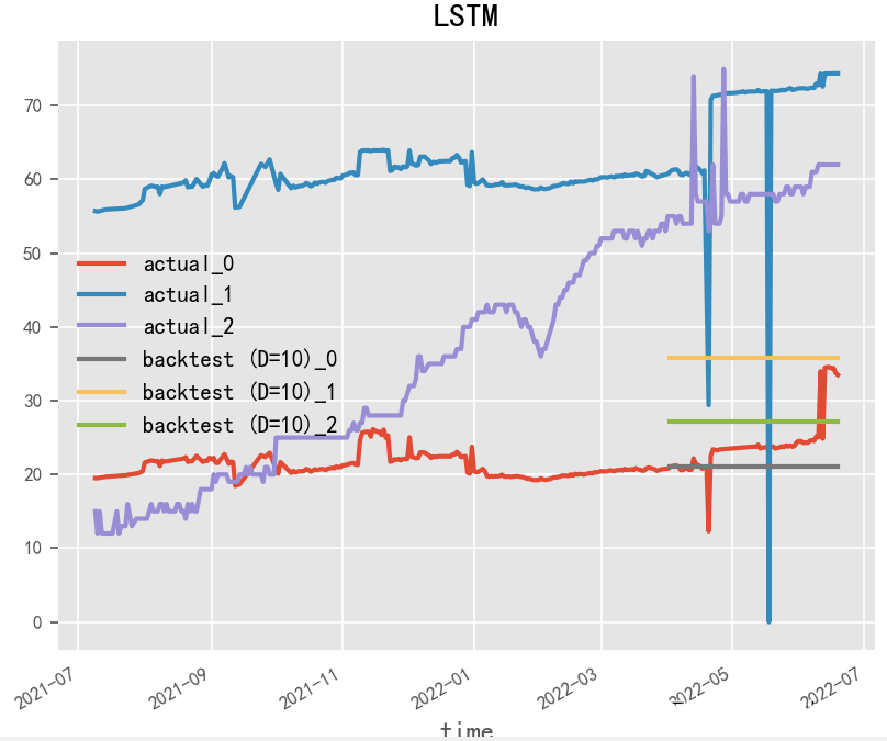
2.1.2 LSTM (1997)

Paper: Long Short-Term Memory

LSTM (Long Short-Term Memory) is a commonly used recurrent neural network model frequently used for time series forecasting. Compared to basic RNN models, LSTM has stronger memory and long-term dependency capabilities, allowing it to better handle the temporal dependencies and dynamic changes in time series data. In constructing LSTM models, the design and parameter tuning of LSTM cells are crucial. The design of LSTM cells can affect the model’s memory capability and long-term dependency ability, while parameter tuning can influence the model’s prediction accuracy and robustness.

# LSTMmodel = RNNModel(    model="LSTM",    hidden_dim=60,    dropout=0,    batch_size=100,    n_epochs=200,    optimizer_kwargs={"lr": 1e-3},    # model_name="Air_RNN",    log_tensorboard=True,    random_state=42,    training_length=20,    input_chunk_length=60,    # force_reset=True,    # save_checkpoints=True,)

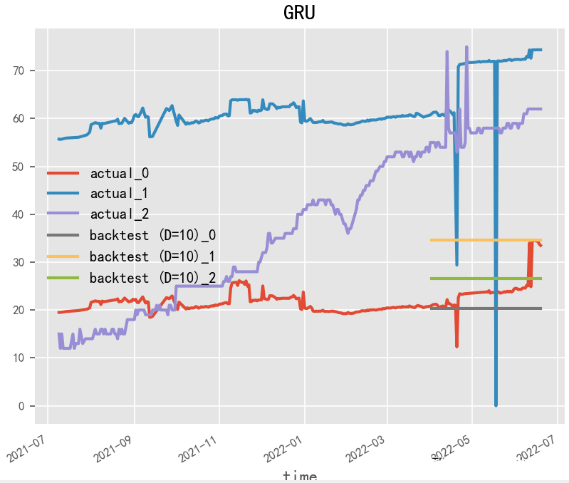
2.1.3 GRU (2014)

Paper: Learning Phrase Representations using RNN Encoder–Decoder for Statistical Machine Translation

GRU (Gated Recurrent Unit) is a commonly used recurrent neural network model, similar to LSTM, specifically designed for handling time series data. Compared to LSTM, the GRU model has fewer parameters and operates faster, yet still effectively manages the temporal dependencies and dynamic changes in time series data. In constructing GRU models, the design and parameter tuning of GRU cells are critical. The design of GRU cells can influence the model’s memory capability and long-term dependency ability, while parameter tuning can affect prediction accuracy and robustness.

# GRUmodel = RNNModel(    model="GRU",    hidden_dim=60,    dropout=0,    batch_size=100,    n_epochs=200,    optimizer_kwargs={"lr": 1e-3},    # model_name="Air_RNN",    log_tensorboard=True,    random_state=42,    training_length=20,    input_chunk_length=60,    # force_reset=True,    # save_checkpoints=True,)

2.1.4 SRU (2018)

Paper: Simple Recurrent Units for Highly Parallelizable Recurrence

SRU (Simple Recurrent Unit) is a recurrent neural network model based on matrix computations, specifically designed for handling time series data. Compared to traditional LSTM and GRU models, SRU has fewer parameters and faster computation speeds while still effectively managing the temporal dependencies and dynamic changes in time series data. In constructing SRU models, the design and parameter tuning of SRU cells are key. The design of SRU cells can affect the model’s memory capability and long-term dependency ability, while parameter tuning can influence prediction accuracy and robustness.

2.2 CNN Class

CNNs can automatically extract features from time series data through convolutional and pooling layers, enabling time series forecasting. When applying CNNs for time series forecasting, it is necessary to convert the time series data into a two-dimensional matrix format, then use convolution and pooling operations for feature extraction and compression, and finally use fully connected layers for prediction. Compared to traditional time series forecasting methods, CNNs can automatically learn complex patterns and rules in time series data while providing better computational efficiency and prediction accuracy.

2.2.1 WaveNet (2016)

Paper: WAVENET: A GENERATIVE MODEL FOR RAW AUDIO

WaveNet is a neural network model proposed by the DeepMind team in 2016 for generating speech. Its core idea is to use convolutional neural networks to simulate the waveform of speech signals and utilize residual connections and gated convolution operations to enhance the model’s representational power. In addition to speech generation, WaveNet can also be applied to time series forecasting tasks. In time series forecasting tasks, we need to predict the value of the next time step for a given time series. Typically, we can view the time series as a one-dimensional vector and input it into the WaveNet model to obtain the predicted value for the next time step.

In constructing WaveNet models, the design and parameter tuning of convolutional layers are crucial. The design of convolutional layers can influence the model’s expressive and generalization abilities, while parameter tuning can affect prediction accuracy and robustness.

2.2.2 TCN (2018)

Paper: An Empirical Evaluation of Generic Convolutional and Recurrent Networks for Sequence Modeling

TCN (Temporal Convolutional Network) is a time series forecasting algorithm based on convolutional neural networks, designed to address the vanishing gradient and high computational complexity problems faced by traditional RNNs when handling long sequences. Compared to traditional RNNs and other sequence models, TCN leverages the characteristics of convolutional neural networks to model long-term dependencies in a shorter time while exhibiting better parallel computing capabilities. The TCN model consists of multiple convolutional layers and residual connections, where the output of each convolutional layer is fed into subsequent convolutional layers to achieve layered abstraction and feature extraction of sequence data. TCN also employs residual connection techniques similar to ResNet, which can effectively reduce issues like vanishing gradients and model degradation, while dilated convolutions can expand the receptive field of the convolution kernel, improving the model’s robustness and accuracy.

The structure of the TCN model is shown in the diagram below:

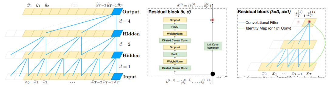
The prediction process of the TCN model includes the following steps:

• Input layer: Receives the input of time series data.
• Convolutional layer: Uses one-dimensional convolution to extract and abstract features from the input data, where each convolutional layer contains multiple convolution kernels that can capture time series patterns at different scales.
• Residual connection: Similar to ResNet, by connecting the output of the convolutional layer with the input via a residual connection, it can effectively reduce issues like vanishing gradients and model degradation, enhancing the model’s robustness.
• Repeated stacking: Repeatedly stack multiple convolutional layers and residual connections to extract abstract features of time series data layer by layer.
• Pooling layer: Add a global average pooling layer after the last convolutional layer to average all feature vectors, resulting in a fixed-length feature vector.

• Output layer: Outputs the prediction values of the time series through a fully connected layer based on the output of the pooling layer.

The advantages of the TCN model include:

• Can handle long sequence data and has good parallelism.
• By introducing techniques such as residual connections and dilated convolutions, it avoids issues like vanishing gradients and overfitting.
• Compared to traditional RNN models, the TCN model has higher computational efficiency and prediction accuracy.

# Model Construction
TCN = TCNModel(    input_chunk_length=13,    output_chunk_length=12,    n_epochs=200,    dropout=0.1,    dilation_base=2,    weight_norm=True,    kernel_size=5,    num_filters=3,    random_state=0,)
# Model Training without Covariates
TCN.fit(series=train,        val_series=val,        verbose=True)
# Model Training with Covariates
TCN.fit(series=train,        past_covariates=train_month,        val_series=val,        val_past_covariates=val_month,        verbose=True)
# Model Inference
backtest = TCN.historical_forecasts(    series=ts,    # past_covariates=month_series,    start=0.75,    forecast_horizon=10,    retrain=False,    verbose=True,)
# Visualization of Results
ts.plot(label="actual")
backtest.plot(label="backtest (D=10)")
plt.legend()
plt.show()

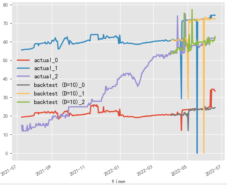
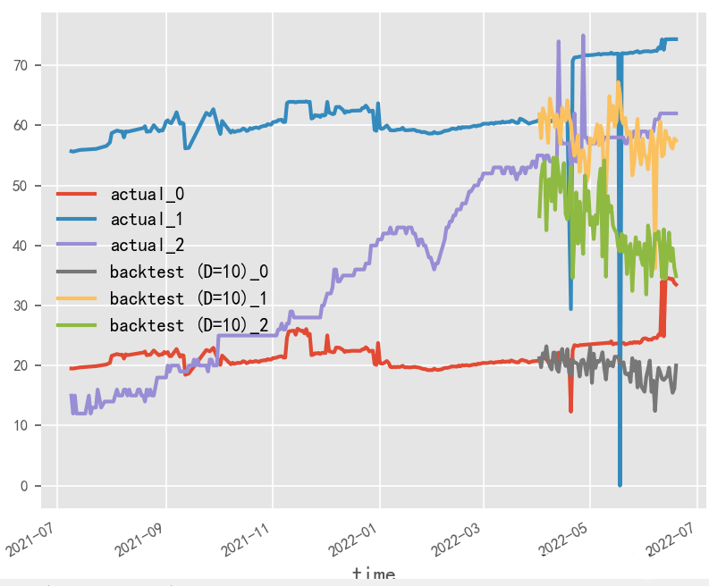
What is the impact of data normalization on time series forecasting?

The original data’s generation of covariates by month and whether normalization is applied have a significant impact on the final time series forecasting results. In this experimental scenario, the original data in percentage format is more suitable for the non-normalized and covariate method, and covariates need to be selected based on actual business performance.

Normalization & No Covariates

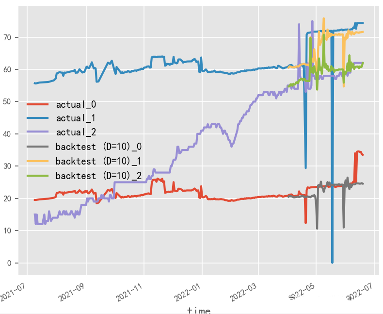
Normalization & With Covariates

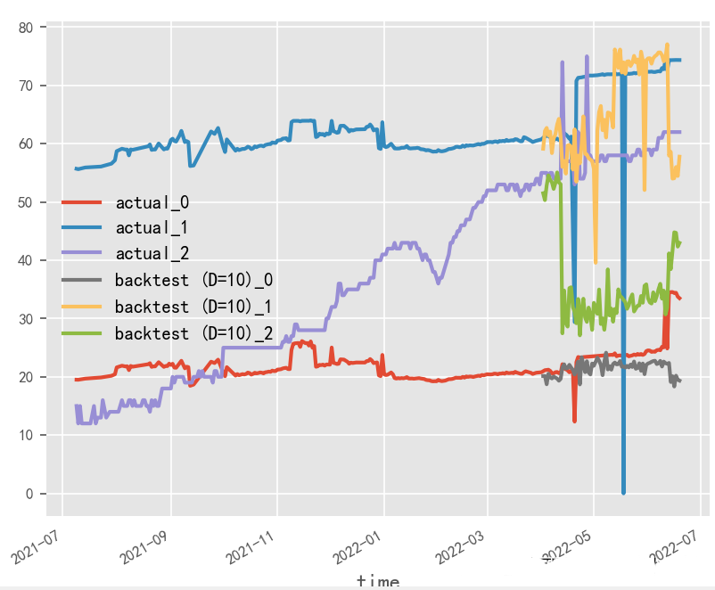
No Normalization & No Covariates

No Normalization & With Covariates

2.2.3 DeepTCN (2019)

Paper: Probabilistic Forecasting with Temporal Convolutional Neural Network. Code: deepTCN

DeepTCN (Deep Temporal Convolutional Networks) is a time series forecasting model based on deep learning, which improves and extends the traditional TCN model. The DeepTCN model uses a set of 1D convolutional layers and max pooling layers to process time series data and extracts different features of time series data by stacking multiple such convolution-pooling layers. In the DeepTCN model, each convolutional layer contains multiple 1D convolution kernels and activation functions and employs residual connections and batch normalization techniques to accelerate model training.

The training process of the DeepTCN model typically involves the following steps:

• Data preprocessing: Standardize and normalize the raw time series data to minimize the impact of inconsistent scales across different features on model training.
• Model construction: Build the DeepTCN model using multiple 1D convolutional layers and max pooling layers, which can be constructed using deep learning frameworks such as TensorFlow, PyTorch, etc.
• Model training: Train the DeepTCN model using the training dataset and measure the model’s prediction performance using loss functions (such as MSE, RMSE, etc.). During training, optimization algorithms (such as SGD, Adam, etc.) can be employed to update model parameters, along with techniques like batch normalization and DeepTCN to enhance the model’s generalization ability.

• Model evaluation: Evaluate the trained DEEPTCN model using the test dataset and calculate performance metrics such as Mean Absolute Error (MAE), Mean Absolute Percentage Error (MAPE), etc.

Exploring the Impact of Input and Output Length on Time Series Forecasting?

In this experimental scenario, due to the limitation of original data samples, the input-output length and batch_size cannot be adjusted too large. From a performance perspective, it is recommended to use a large batch_size and short input-output method.

# Short Input and Output
deeptcn = TCNModel(    input_chunk_length=13,    output_chunk_length=12,    kernel_size=2,    num_filters=4,    dilation_base=2,    dropout=0.1,    random_state=0,    likelihood=GaussianLikelihood(),)
# Long Input and Output
deeptcn = TCNModel(    input_chunk_length=60,    output_chunk_length=20,    kernel_size=2,    num_filters=4,    dilation_base=2,    dropout=0.1,    random_state=0,    likelihood=GaussianLikelihood(),)
# Long Input and Output, Large Batch Size
deeptcn = TCNModel(    batch_size=60,    input_chunk_length=60,    output_chunk_length=20,    kernel_size=2,    num_filters=4,    dilation_base=2,    dropout=0.1,    random_state=0,    likelihood=GaussianLikelihood(),)
# Short Input and Output, Large Batch Size
deeptcn = TCNModel(    batch_size=60,    input_chunk_length=13,    output_chunk_length=12,    kernel_size=2,    num_filters=4,    dilation_base=2,    dropout=0.1,    random_state=0,    likelihood=GaussianLikelihood(),)

Short Input and Output

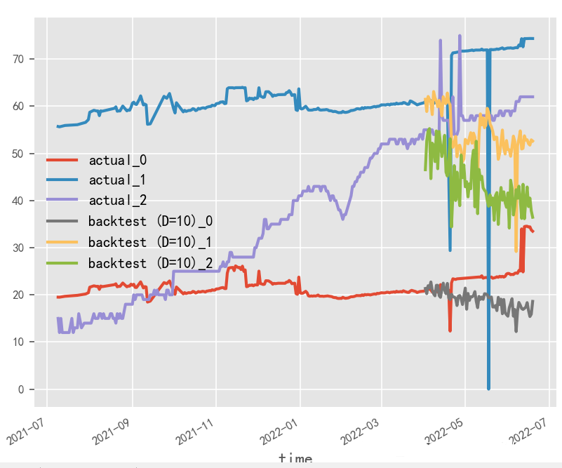
Long Input and Output

Long Input and Output, Large Batch Size

Short Input and Output, Large Batch Size

2.3 Attention Class

The Attention mechanism is used to address the extraction of important features in sequence input data and has also been applied in the field of time series forecasting. The Attention mechanism can automatically focus on important parts of time series data, providing the model with more useful information, thereby improving prediction accuracy. When applying Attention for time series forecasting, it is necessary to use the Attention mechanism to adaptively weight different parts of the input data, allowing the model to focus more on key information while reducing the impact of irrelevant information. The Attention mechanism can be applied not only to RNNs and other sequence models but also to CNNs and other non-sequence models, making it one of the hot research topics in the field of time series forecasting.

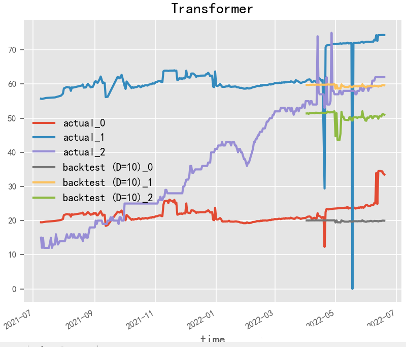
2.3.1 Transformer (2017)

Paper: Attention Is All You Need

Transformer is a neural network model widely used in the field of Natural Language Processing (NLP), essentially functioning as a sequence-to-sequence (seq2seq) model. The Transformer treats each position in the sequence as a vector and uses multi-head self-attention mechanisms and feedforward neural networks to capture long-range dependencies in the sequence, enabling the model to handle variable-length and indefinite-length sequences.

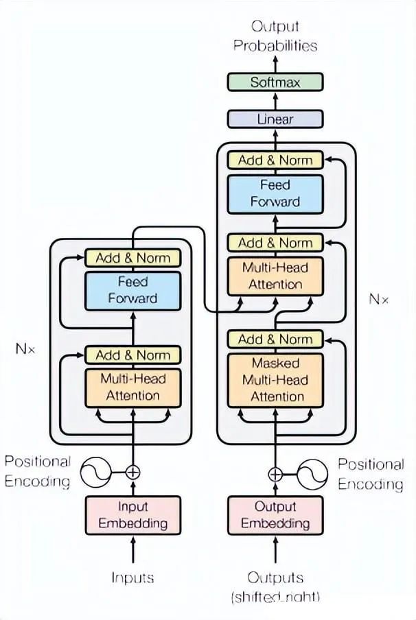
In time series forecasting tasks, the Transformer model can treat the time steps of the input sequence as positional information, represent the features of each time step as a vector, and use an encoder-decoder framework for prediction. Specifically, the first N time steps of the prediction target can be used as the input to the encoder, while the subsequent M time steps can be used as the input to the decoder, employing the encoder-decoder framework for prediction. Both the encoder and decoder are composed of multiple stacked Transformer modules, with each module consisting of multi-head self-attention layers and feedforward neural network layers.

During training, common loss functions such as Mean Squared Error (MSE) or Mean Absolute Error (MAE) can be used to measure the model’s prediction performance, and optimization algorithms such as Stochastic Gradient Descent (SGD) or Adam can be employed to update model parameters. During model training, techniques such as learning rate adjustment and gradient clipping can also be utilized to accelerate training and improve model performance.

# Transformermodel = TransformerModel(    input_chunk_length=30,    output_chunk_length=15,    batch_size=32,    n_epochs=200,    # model_name="air_transformer",    nr_epochs_val_period=10,    d_model=16,    nhead=8,    num_encoder_layers=2,    num_decoder_layers=2,    dim_feedforward=128,    dropout=0.1,    optimizer_kwargs={"lr": 1e-2},    activation="relu",    random_state=42,    # save_checkpoints=True,    # force_reset=True,)

2.3.2 TFT (2019)

Paper: Temporal Fusion Transformers for Interpretable Multi-horizon Time Series Forecasting

TFT (Transformer-based Time Series Forecasting) is a time series forecasting method based on the Transformer model, proposed by the Google DeepMind team in 2019. The core idea of the TFT method is to introduce temporal feature embeddings and modality embeddings into the Transformer model. Temporal feature embeddings help the model better learn features such as periodicity and trends in time series data, while modality embeddings allow external influencing factors (such as temperature, holidays, etc.) to be predicted alongside time series data.

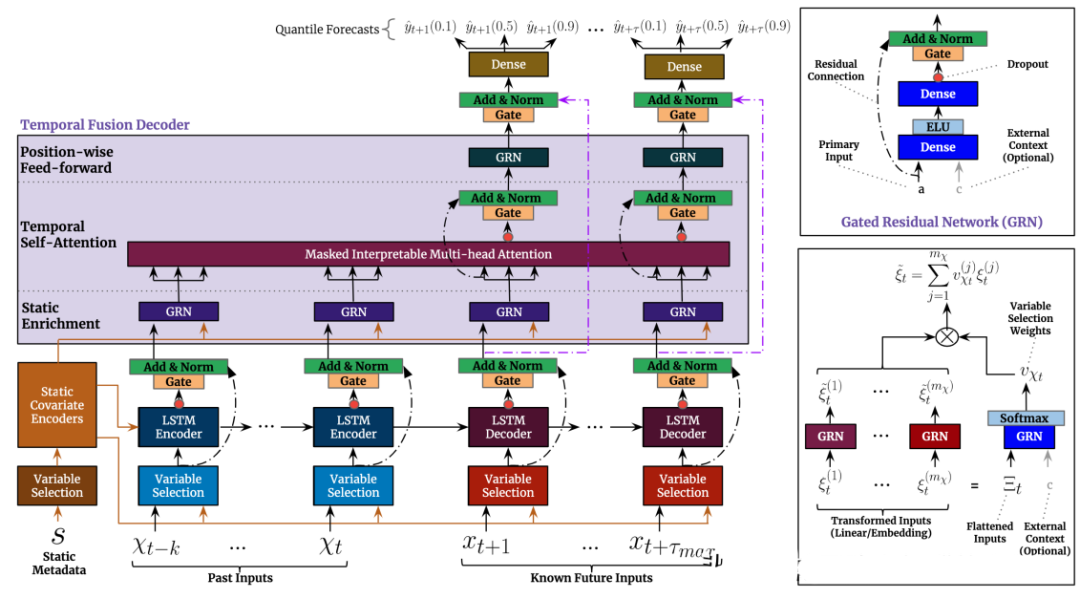
The TFT method can be divided into two phases: the training phase and the prediction phase. In the training phase, the TFT method uses training data to train the Transformer model and employs techniques such as random masking and adaptive learning rate adjustment to enhance the model’s robustness and training efficiency. In the prediction phase, the TFT method utilizes the trained model to forecast future time series data.

Compared to traditional time series forecasting methods, the TFT method has the following advantages:

• Can better handle time series data at different scales because the Transformer model can learn both global and local features of time series.
• Can simultaneously consider time series data and external influencing factors, improving prediction accuracy.

• Can directly learn the prediction model through an end-to-end training approach without the need for manual feature extraction.

# TFTmodel = TransformerModel(    input_chunk_length=30,    output_chunk_length=15,    batch_size=32,    n_epochs=200,    # model_name="air_transformer",    nr_epochs_val_period=10,    d_model=16,    nhead=8,    num_encoder_layers=2,    num_decoder_layers=2,    dim_feedforward=128,    dropout=0.1,    optimizer_kwargs={"lr": 1e-2},    activation="relu",    random_state=42,    # save_checkpoints=True,    # force_reset=True,)

2.3.3 HT (2019)

HT (Hierarchical Transformer) is a time series forecasting algorithm based on the Transformer model, proposed by researchers from the Chinese University of Hong Kong. The HT model employs a hierarchical structure to process time series data with multiple time scales and uses an adaptive attention mechanism to capture features at different time scales, enhancing the model’s prediction performance and generalization capability.

The HT model consists of two main components: the multi-scale attention module and the prediction module. In the multi-scale attention module, the HT model captures features at different time scales through an adaptive multi-head attention mechanism and fuses features from different time scales into a common feature representation. In the prediction module, the HT model uses fully connected layers to predict the feature representation and outputs the final prediction result.

The advantages of the HT model are that it can adaptively handle time series data with multiple time scales and capture features at different time scales through an adaptive multi-head attention mechanism, enhancing the model’s prediction performance and generalization capability. Additionally, the HT model has good interpretability and generalization ability, making it suitable for various time series forecasting tasks.

2.3.4 LogTrans (2019)

Paper: Enhancing the Locality and Breaking the Memory Bottleneck of Transformer on Time Series Forecasting

Code: Autoformer

LogTrans proposes an improved method for Transformer time series forecasting, including convolutional self-attention (which generates queries and keys with causal convolutions, incorporating local environments into the attention mechanism) and LogSparse Transformer (a memory-efficient variant of Transformer used to reduce memory costs for modeling long time series), primarily addressing the two main weaknesses of Transformer time series forecasting: position-independent attention and memory bottlenecks.

2.3.5 DeepTTF (2020)

DeepTTF (Deep Temporal Transformational Factorization) is a time series forecasting algorithm based on deep learning and matrix factorization, proposed by researchers from UCLA. The DeepTTF model decomposes time series into multiple time segments and uses matrix factorization techniques to model each time segment to enhance the model’s prediction performance and interpretability.

The DeepTTF model consists of three main components: time segmentation, matrix factorization, and predictor. In the time segmentation phase, the DeepTTF model divides the time series into multiple segments, each containing a continuous period. In the matrix factorization phase, the DeepTTF model decomposes each time segment into two low-dimensional matrices representing the relationship between time and features. In the predictor phase, the DeepTTF model uses multilayer perceptrons to predict each time segment and combines the prediction results into the final prediction sequence.

The advantages of the DeepTTF model are that it can effectively capture local patterns and global trends in time series while maintaining high prediction accuracy and interpretability. Additionally, the DeepTTF model supports time-segment-based cross-validation to enhance the model’s robustness and generalization capability.

2.3.6 PTST (2020)

Probabilistic Time Series Transformer (PTST) is a time series forecasting algorithm based on the Transformer model, proposed by Google Brain in 2020. This algorithm employs probabilistic graphical models to improve the accuracy and reliability of time series forecasting, achieving better performance in time series data with high uncertainty.

The PTST model consists of two parts: the sequence model and the probability model. The sequence model uses the Transformer structure to encode and decode time series data and employs self-attention mechanisms to focus on and extract important information from the sequence. The probability model introduces variational autoencoders (VAE) and Kalman filters (KF) to capture uncertainties and noise in time series data.

Specifically, the PTST model’s sequence model uses a Transformer Encoder-Decoder structure for time series forecasting. The Encoder part employs multi-layer self-attention mechanisms to extract features from the input sequence, while the Decoder part generates the output sequence step by step through autoregression. On this basis, the probability model introduces a random variable, the noise term of the time series data, which is modeled as a normal distribution. Additionally, to minimize potential errors, the probability model also uses KF for smoothing the sequence.

During training, PTST uses the Maximum A Posteriori (MAP) estimation method to maximize the predicted probabilities. In the prediction phase, PTST utilizes Monte Carlo sampling methods to sample from the posterior distribution to generate a set of probability distributions. To measure the prediction accuracy, PTST also incorporates loss functions such as Mean Squared Error and Negative Log Likelihood (NLL).

2.3.7 Reformer (2020)

Paper: Reformer: The Efficient Transformer

Reformer is a neural network structure based on the Transformer model, which has certain application prospects in time series forecasting tasks. The Reformer model can be used for sampling, autoregression, multi-step forecasting, and combining reinforcement learning methods for time series forecasting. In these methods, known historical time steps are input into the model, which then generates values for future time steps. The Reformer model enhances efficiency, accuracy, and scalability by introducing separable convolutions and reversible layers. In summary, the Reformer model provides a new perspective and method for time series forecasting tasks.

2.3.8 Informer (2020)

Paper: Informer: Beyond Efficient Transformer for Long Sequence Time-Series Forecasting

Code: https://github.com/zhouhaoyi/Informer2020

Informer is a time series forecasting method based on the Transformer model, proposed by the Deep Learning and Computational Intelligence Laboratory at Peking University in 2020. Unlike traditional Transformer models, Informer introduces a new structure and mechanisms to better adapt to time series forecasting tasks. The core ideas of the Informer method include:

• Long Short-Term Memory (LSTM) encoder-decoder structure: Informer incorporates an LSTM encoder-decoder structure to alleviate long-term dependency issues in time series to some extent.
• Adaptive Length Attention (AL) mechanism: Informer proposes an adaptive length attention mechanism to capture important information in sequences at different time scales.
• Multi-Scale Convolution Kernel (MSCK) mechanism: Informer uses a multi-scale convolution kernel mechanism to simultaneously consider features at different time scales.

• Generative Adversarial Network (GAN) framework: Informer employs a GAN framework to further enhance the model’s prediction accuracy through adversarial learning.

During the training phase, the Informer method can utilize various loss functions (such as Mean Absolute Error, Mean Squared Error, L1-Loss, etc.) to train the model and use the Adam optimization algorithm to update model parameters. In the prediction phase, the Informer method can employ sliding window techniques to forecast the values of future time points.

Experiments have been conducted on multiple time series forecasting datasets using the Informer method, and comparisons have been made with other popular time series forecasting methods. Experimental results indicate that the Informer method demonstrates excellent performance in terms of prediction accuracy, training speed, and computational efficiency.

2.3.9 TAT (2021)

TAT (Temporal Attention Transformer) is a time series forecasting algorithm based on the Transformer model, proposed by the Intelligent Science Laboratory at Peking University. The TAT model enhances the traditional Transformer model by introducing a temporal attention mechanism, which better captures dynamic changes in time series.

The basic structure of the TAT model is similar to that of the Transformer, consisting of multiple Encoder and Decoder layers. Each Encoder layer includes a multi-head self-attention mechanism and a feedforward network to extract features from the input sequence. Each Decoder layer includes a multi-head self-attention mechanism, multi-head attention mechanism, and feedforward network to generate the output sequence step by step. Unlike traditional Transformer models, the TAT model introduces a temporal attention mechanism in the multi-head attention mechanism to capture dynamic changes in time series. Specifically, the TAT model inputs time step information as an additional feature and uses the multi-head attention mechanism to focus on and extract time steps, aiding the model in modeling dynamic changes in the sequence. Additionally, the TAT model employs incremental training techniques to improve training efficiency and prediction performance.

2.3.10 NHT (2021)

Paper: Nested Hierarchical Transformer: Towards Accurate, Data-Efficient and Interpretable Visual Understanding

NHT (Nested Hierarchical Transformer) is a deep learning algorithm for time series forecasting. It adopts a nested hierarchical transformer structure, utilizing nested self-attention mechanisms and time importance evaluation mechanisms at multiple levels to achieve accurate predictions of time series data. The NHT model improves the traditional self-attention mechanism by introducing more hierarchical structures, while dynamically controlling the importance of different levels through time importance evaluation mechanisms to achieve better prediction performance. This algorithm has demonstrated excellent performance across various time series forecasting tasks, proving its potential in the field of time series forecasting.

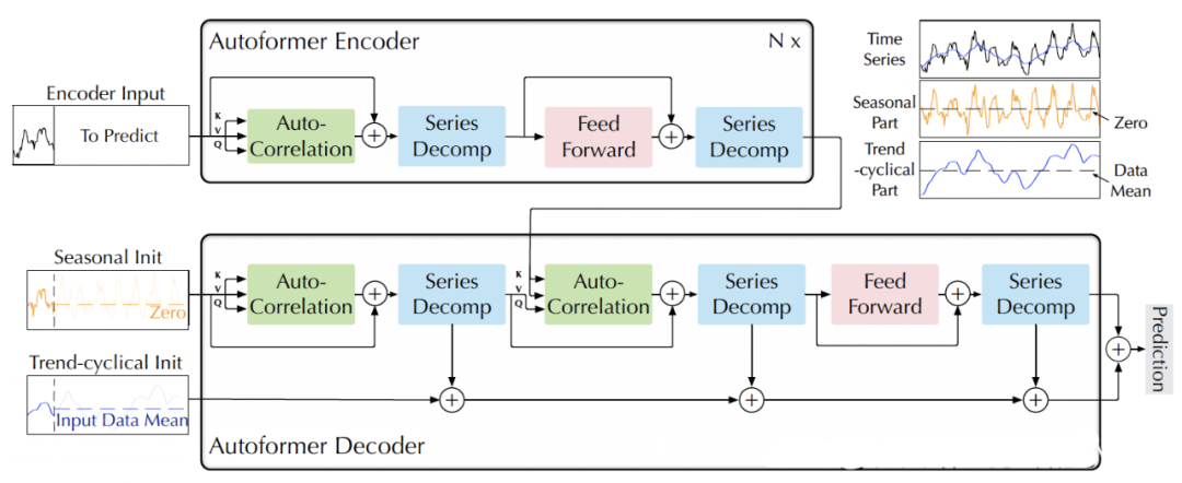
2.3.11 Autoformer (2021)

Paper: Autoformer: Decomposition Transformers with Auto-Correlation for Long-Term Series

Forecasting Code: https://github.com/thuml/Autoformer

AutoFormer is a time series forecasting model based on the Transformer structure. Compared to traditional RNN, LSTM, and other models, AutoFormer has the following features:

• Self-attention mechanism: AutoFormer employs a self-attention mechanism to capture both global and local relationships in time series, avoiding the vanishing gradient problem during long sequence training.
• Transformer structure: AutoFormer utilizes the Transformer structure to enable parallel computing, enhancing training efficiency.

• Multi-task learning: AutoFormer supports multi-task learning, allowing simultaneous predictions of multiple time series, improving the model’s efficiency and accuracy.

The specific structure of the AutoFormer model is similar to that of the Transformer, consisting of encoder and decoder components. The encoder is composed of multiple self-attention layers and feedforward neural network layers to extract features from the input sequence. The decoder also consists of multiple self-attention layers and feedforward neural network layers to convert the encoder’s output into the prediction sequence. Additionally, AutoFormer introduces cross-time-step attention mechanisms to adaptively select time steps in both the encoder and decoder. Overall, AutoFormer is an efficient and accurate time series forecasting model suitable for various types of time series forecasting tasks.

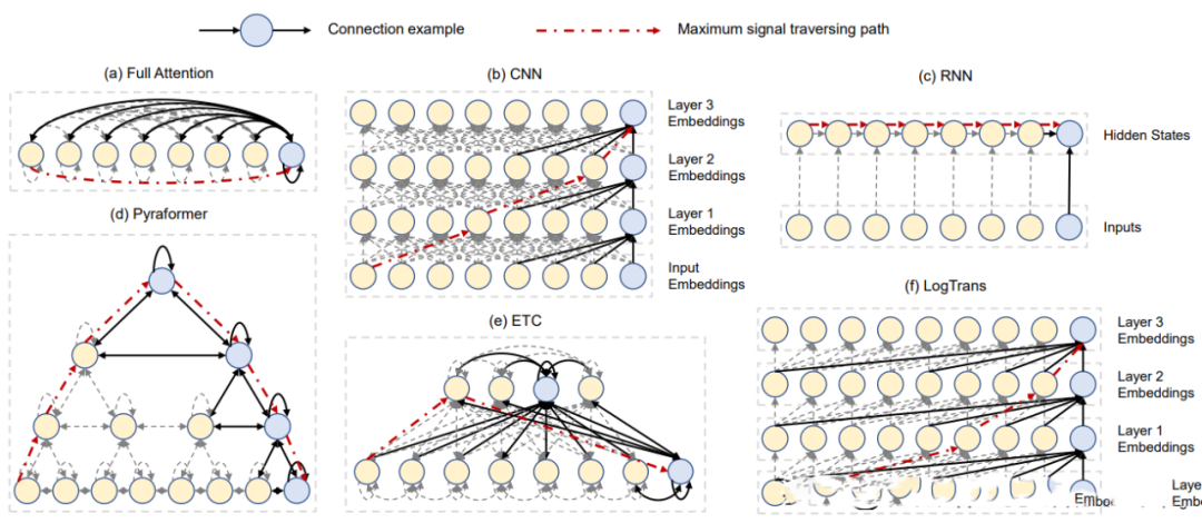
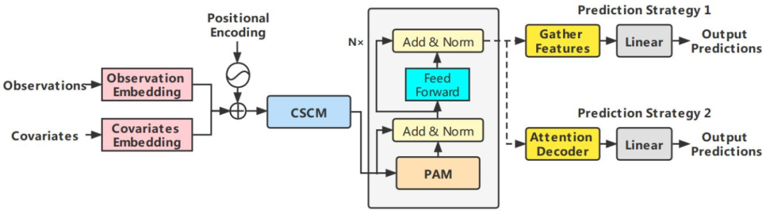
2.3.12 Pyraformer (2022)

Paper: Pyraformer: Low-complexity Pyramidal Attention for Long-range Time Series Modeling and Forecasting Code: https://github.com/ant-research/Pyraformer

Ant Research Institute proposed a new Transformer (Pyraformer) based on pyramidal attention to bridge the gap between capturing long-range dependencies and achieving low temporal and spatial complexity. Specifically, it develops a pyramidal attention mechanism by passing attention-based information in a pyramid graph, as illustrated in the figure (d). The edges in the graph can be divided into two groups: inter-scale connections and intra-scale connections. Inter-scale connections build a multi-resolution representation of the original sequence: nodes at the finest scale correspond to time points in the original time series (e.g., hourly observations), while nodes at coarser scales represent lower-resolution features (e.g., daily, weekly, and monthly patterns).

These potential coarse-scale nodes are initially introduced through a coarse-scale construction module. On the other hand, intra-scale edges connect adjacent nodes to capture temporal correlations at each resolution. Thus, the model provides a concise representation of long-term temporal dependencies between distant locations by capturing such behaviors at coarser resolutions, significantly reducing computational costs.

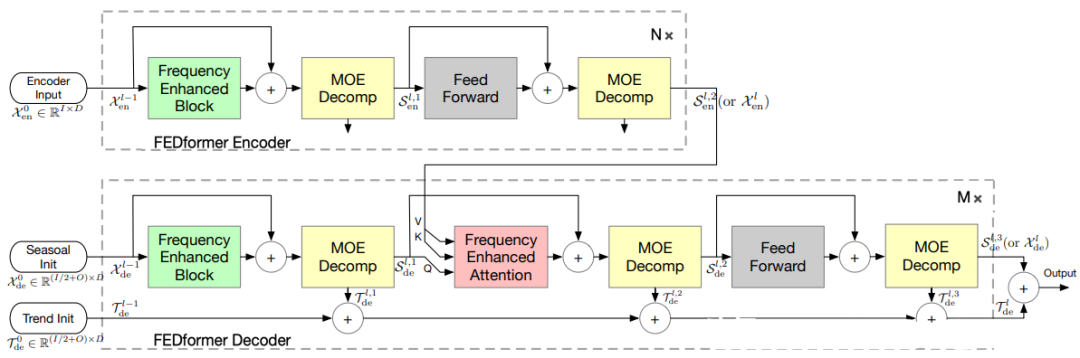
2.3.13 FEDformer (2022)

Paper: FEDformer: Frequency Enhanced Decomposed Transformer for Long-term Series

Forecasting Code: https://github.com/MAZiqing/FEDformer

FEDformer is a neural network structure based on the Transformer model, specifically designed for distributed time series forecasting tasks. This model divides time series data into multiple small chunks and accelerates the training process through distributed computing. FEDformer introduces local attention mechanisms and reversible attention mechanisms, enabling the model to better capture local features in time series data while achieving higher computational efficiency. Additionally, FEDformer supports dynamic partitioning, asynchronous training, and adaptive chunking, providing the model with greater flexibility and scalability.

2.3.14 Crossformer (2023)

Paper: Crossformer: Transformer Utilizing Cross-Dimension Dependency for Multivariate Time Series

Forecasting Code: https://github.com/Thinklab-SJTU/Crossformer

Crossformer proposes a new hierarchical Encoder-Decoder architecture, consisting of a left-side Encoder (gray) and a right-side Decoder (light orange), including Dimension-Segment-Wise (DSW) embedding, Two-Stage Attention (TSA) layers, and Linear Projection.

2.4 Mix Class

Combining ETS, autoregression, RNN, CNN, and Attention algorithms can utilize their respective advantages to improve the accuracy and stability of time series forecasting. This combination method is commonly referred to as a “mixed model.” Among them, RNN can automatically learn long-term dependencies in time series data; CNN can automatically extract local and spatial features from time series data; and the Attention mechanism can adaptively focus on important parts of time series data. By merging these algorithms, time series forecasting models can become more robust and accurate. In practical applications, suitable algorithm combination methods can be selected based on different time series forecasting scenarios, followed by model tuning and optimization.

2.4.1 Encoder-Decoder CNN (2017)

Paper: Deep Learning for Precipitation Nowcasting: A Benchmark and A New Model

Encoder-Decoder CNN is also a model that can be used for time series forecasting tasks; it is a convolutional neural network that integrates both encoder and decoder. In this model, the encoder is used to extract features from the time series, while the decoder generates future time series.

Specifically, the Encoder-Decoder CNN model can follow these steps for time series forecasting:

• Input historical time series data and extract features through convolutional layers.
• Feed the feature sequence output from the convolutional layer into the encoder, gradually reducing the feature dimensions through pooling operations while retaining the encoder’s state vector.
• Feed the encoder’s state vector into the decoder, generating future time series data step by step through deconvolution and upsampling operations.

• Post-process the decoder’s output, such as de-mean or normalize, to obtain the final prediction result.

It should be noted that the Encoder-Decoder CNN model requires appropriate loss functions (such as Mean Squared Error or Cross-Entropy) during training and hyperparameter adjustments as needed. Additionally, to enhance the model’s generalization ability, techniques such as cross-validation should be used for model evaluation and selection.

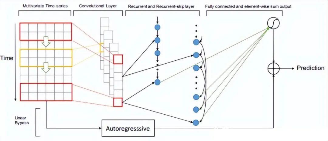
2.4.2 LSTNet (2018)

Paper: Modeling Long- and Short-Term Temporal Patterns with Deep Neural Networks

LSTNet is a deep learning model for time series forecasting, officially known as Long- and Short-term Time-series Networks. LSTNet combines Long Short-Term Memory networks (LSTM) and one-dimensional convolutional neural networks (1D-CNN) to effectively handle both long-term and short-term time series information while capturing seasonal and cyclical changes in the sequence. LSTNet was initially proposed in 2018 by Guokun Lai and others from the Institute of Computing Technology, Chinese Academy of Sciences.

The core idea of the LSTNet model is to use CNN for feature extraction from time series data and then input the extracted features into LSTM for sequence modeling. LSTNet also includes an adaptive weight learning mechanism that effectively balances the importance of long-term and short-term time series information. The input to the LSTNet model is a time series matrix with a shape of (T, d), where T represents the number of time steps and d represents the feature dimension at each time step. The output of LSTNet is a prediction vector of length H, where H represents the number of predicted time steps. During training, LSTNet employs Mean Squared Error (MSE) as the loss function and optimizes using backpropagation.

2.4.3 TDAN (2018)

Paper: TDAN: Temporal Difference Attention Network for Precipitation Nowcasting

TDAN (Time-aware Deep Attentive Network) is a deep learning algorithm for time series forecasting that integrates convolutional neural networks and attention mechanisms to capture the temporal features of time series. Compared to traditional convolutional neural networks, TDAN can more effectively utilize the temporal information in time series data, thereby improving prediction accuracy.

Specifically, the TDAN algorithm can follow these steps for time series forecasting:

• Input historical time series data and extract features through convolutional layers.
• Feed the feature sequence output from the convolutional layers into the attention mechanism, calculating the weighted feature vector based on the weights related to the current prediction from historical data.
• Feed the weighted feature vector into fully connected layers for the final prediction.

It should be noted that the TDAN algorithm requires appropriate loss functions (such as Mean Squared Error) during training and hyperparameter adjustments as needed. Additionally, to enhance the model’s generalization ability, techniques such as cross-validation should be used for model evaluation and selection.

The advantages of the TDAN algorithm lie in its ability to adaptively focus on parts of historical data relevant to the current prediction, thereby improving prediction accuracy. It can also effectively handle missing values and outliers in time series data, demonstrating a certain level of robustness.

2.4.4 DeepAR (2019)

Paper: DeepAR: Probabilistic Forecasting with Autoregressive Recurrent Networks

DeepAR is an autoregressive recurrent neural network that uses recurrent neural networks (RNN) combined with autoregressive AR to predict scalar (one-dimensional) time series. In many applications, there are multiple similar time series across a representative set of units. DeepAR combines multiple similar time series, such as sales data for different flavors of instant noodles, learning the internal correlation characteristics among different time series through deep recurrent neural networks, using multivariate or multiple target counts to enhance overall prediction accuracy. DeepAR ultimately generates multi-step prediction results for an optional time span, with single time point predictions being probabilistic, typically outputting P10, P50, and P90 values. Here, P10 refers to the probability distribution indicating a 10% chance of being below P10.

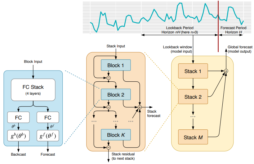
2.4.5 N-BEATS (2020)

Paper: N-BEATS: Neural basis expansion analysis for interpretable time series

Forecasting Code: https://github.com/amitesh863/nbeats_forecast

N-BEATS (Neural basis expansion analysis for interpretable time series forecasting) is a time series forecasting model based on neural networks, developed by Oriol Vinyals and others in the Google Brain team. N-BEATS uses learned basis functions to represent time series data, achieving high accuracy while enhancing model interpretability. The N-BEATS model employs stacked regression modules and inverse convolution modules to effectively handle multi-scale time series data and long-term dependencies.

model = NBEATSModel(    input_chunk_length=30,    output_chunk_length=15,    n_epochs=100,    num_stacks=30,    num_blocks=1,    num_layers=4,    dropout=0.0,    activation='ReLU')

2.4.6 TCN-LSTM (2021)

Paper: A Comparative Study of Detecting Anomalies in Time Series Data Using LSTM and TCN Models

TCN-LSTM is a model that integrates Temporal Convolutional Network (TCN) and Long Short-Term Memory (LSTM), suitable for time series forecasting tasks. In this model, TCN layers and LSTM layers collaborate to capture features of long-term and short-term time series, respectively. Specifically, the TCN layer can be implemented by stacking multiple convolutional layers to expand the receptive field while preventing gradient vanishing through residual connections. The LSTM layer captures the long-term dependencies in time series through memory cells and gating mechanisms.

The TCN-LSTM model can follow these steps for time series forecasting:

• Input historical time series data and extract short-term features through TCN layers.
• Feed the feature sequence output from the TCN layer into the LSTM layer to capture the long-term dependencies in the time series.
• Feed the feature vector output from the LSTM layer into fully connected layers for the final prediction.

It should be noted that the TCN-LSTM model requires appropriate loss functions (such as Mean Squared Error) during training and hyperparameter adjustments as needed. Additionally, to enhance the model’s generalization ability, techniques such as cross-validation should be used for model evaluation and selection.

2.4.7 NeuralProphet (2021)

Paper: Neural Forecasting at Scale

NeuralProphet is a neural network-based time series forecasting framework provided by Facebook, which builds upon the Prophet framework by adding some neural network structures to more accurately forecast time series data with complex nonlinear trends and seasonality.

• The core idea of NeuralProphet is to utilize deep neural networks to learn the nonlinear features of time series and combine the decomposition model of Prophet with neural networks. NeuralProphet offers various neural network structures and optimization algorithms that can be selected and adjusted based on specific application needs. The features of NeuralProphet include:
• Flexibility: NeuralProphet can handle time series data with complex trends and seasonality and allows flexible configuration of neural network structures and optimization algorithms.
• Accuracy: NeuralProphet can leverage the nonlinear modeling capabilities of neural networks to improve the accuracy of time series forecasting.
• Interpretability: NeuralProphet provides rich visualization tools to help users understand prediction results and influencing factors.

• Usability: NeuralProphet can be easily integrated with programming languages like Python and offers rich APIs and examples, allowing users to quickly get started.

NeuralProphet has wide applications in many fields, such as finance, transportation, and electricity. It can assist users in predicting future trends and variations in trends, providing useful references and decision support.

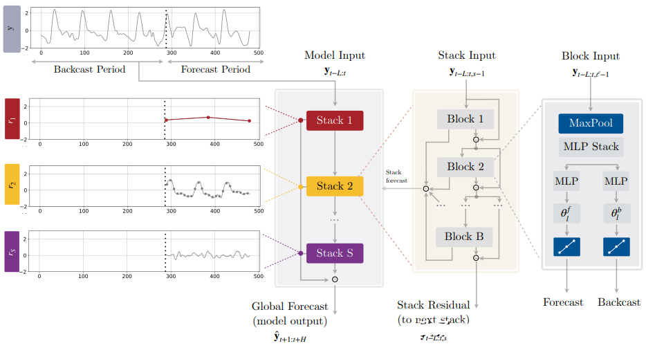
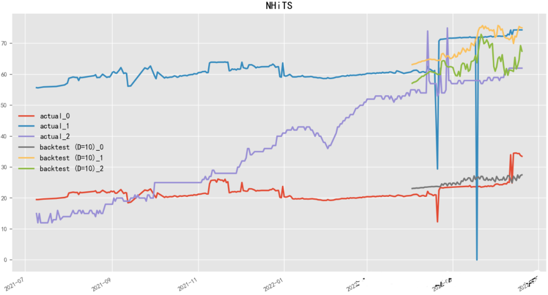
2.4.8 N-HiTS (2022)

Paper: N-HiTS: Neural Hierarchical Interpolation for Time Series Forecasting

N-HiTS (Neural network-based Hierarchical Time Series) is a hierarchical time series forecasting model based on neural networks, developed by the Uber team. N-HiTS employs deep learning methods to predict multi-level time series data, such as product sales, traffic, stock prices, etc. The model adopts a hierarchical structure, decomposing the entire time series data into multiple hierarchies, each containing different time granularities and features, and then uses neural network models for prediction. N-HiTS also employs an adaptive learning algorithm that can dynamically adjust the structure and parameters of the prediction model to maximize prediction accuracy.

model = NHiTSModel(    input_chunk_length=30,    output_chunk_length=15,    n_epochs=100,    num_stacks=3,    num_blocks=1,    num_layers=2,    dropout=0.1,    activation='ReLU')

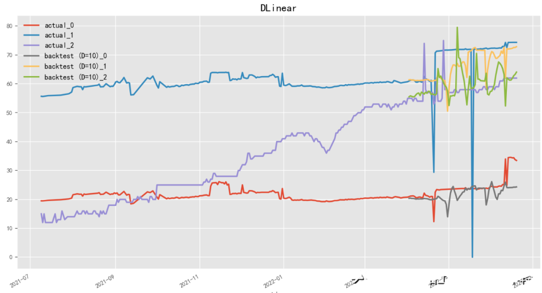
2.4.9 D-Linear (2022)

Paper: Are Transformers Effective for Time Series Forecasting?

Code: https://github.com/cure-lab/LTSF-Linear

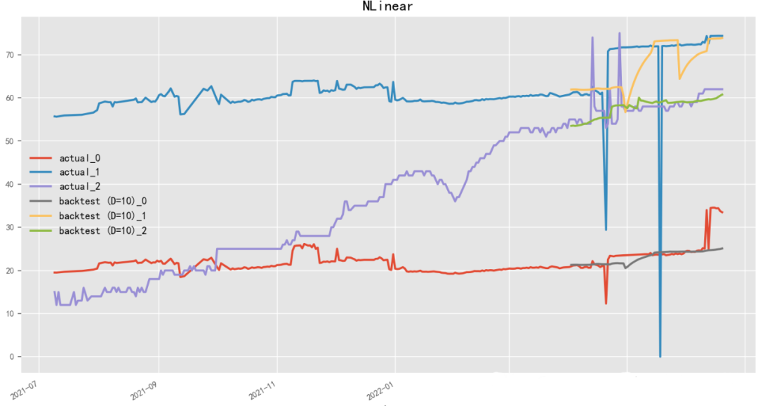
D-Linear (Deep Linear Model) is a linear time series forecasting model based on neural networks, developed by the Li Hongyi team. D-Linear uses neural network structures for linear prediction of time series data, achieving high prediction accuracy while enhancing the model’s interpretability. The model employs a Multilayer Perceptron as the neural network model and improves model performance through alternating training and fine-tuning. D-Linear also provides a feature selection method based on sparse coding, automatically selecting features with discriminative and predictive capabilities. Similarly, N-Linear (Neural Linear Model) is a linear time series forecasting model based on neural networks, developed by the Baidu team.

model = DLinearModel(    input_chunk_length=15,    output_chunk_length=13,    batch_size=90,    n_epochs=100,    shared_weights=False,    kernel_size=25,    random_state=42)
model = NLinearModel(    input_chunk_length=15,    output_chunk_length=13,    batch_size=90,    n_epochs=100,    shared_weights=True,    random_state=42)