
Click on the above “Beginner Learning Vision”, select “Star” or “Top”
Important content delivered first time
With the rapid development of artificial intelligence, especially deep learning, computer vision has become a particularly popular research direction in recent years. Here, we will launch a brand new series 【Computer Vision Insights】 to share some of our understanding and experiences in computer vision over the years. In this series, we will mainly focus on deep learning algorithms in computer vision, covering various fields such as image classification, object detection, image segmentation, and video understanding.
Now we begin the first article of this series, in which we will provide an in-depth introduction to the basic knowledge of deep learning, specifically focusing on deep neural networks, hoping to walk step by step into the world of computer vision from scratch.
Before discussing deep learning, let’s first review the perceptron model. The perceptron is the origin algorithm of deep neural networks, and learning and mastering the perceptron is a necessary path to deep learning.
The perceptron is the first neural network model that is completely described algorithmically, and it is one of the simplest models applied to binary classification tasks. The model’s input is the feature vector of the sample, and the output is the category of the sample, represented by 1 and -1 respectively. The goal of the perceptron is to separate the samples in the input space (feature space) into positive and negative classes using a separating hyperplane, mathematically described as follows:
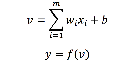
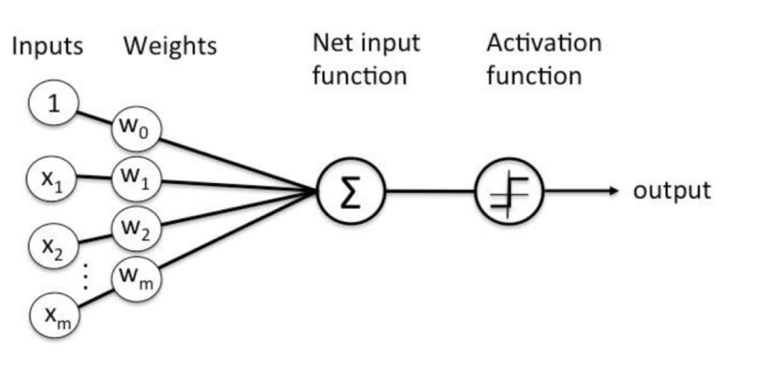
Where, wi represents the weight corresponding to the i-th feature xi of the input sample, b represents the bias of the model, f represents the activation function, using the sign step function here, which outputs 1 if greater than 0, otherwise -1, and y represents the predicted label of the input sample.
In practical applications, the weights w and bias b need to be updated through multiple iterations during the training process. For convenience, we use X to represent the input features and W to represent the weight matrix, rewriting X and W as follows:
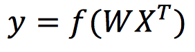
Thus, the perceptron can be rewritten as

The intuitive computation process is shown in the following figure.
During the training of the perceptron, we continuously correct the weights for misclassified samples, iterating gradually until the final classification meets the predetermined criteria, thus determining the weights. Specifically, we generally use a loss function based on misclassification to update the weights through the gradient descent algorithm, as shown in the following equation:
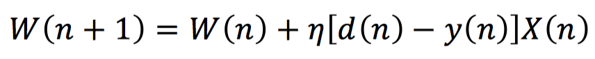
Where, d(n) represents the actual label corresponding to the n-th input X(n), y(n) represents the predicted label output by the perceptron during the n-th input, and η represents the learning rate.
For example, in binary classification of images, assuming we already have the features x of each image and their corresponding categories y, we can quickly build a binary classification model for images using the perceptron introduced above. However, the perceptron can only determine one hyperplane during classification, suitable for handling linearly separable problems but not good at complex nonlinear scenarios.
In the previous section, we introduced a single perceptron for handling simple binary classification data. In this section, we will transition from a single perceptron to a multi-layer perceptron (MLP). The multi-layer perceptron is a classic neural network model that can be widely applied to complex nonlinear classification scenarios. The following figure shows a typical multi-layer perceptron, also known as a fully connected neural network, where each blue neuron represents a perceptron.
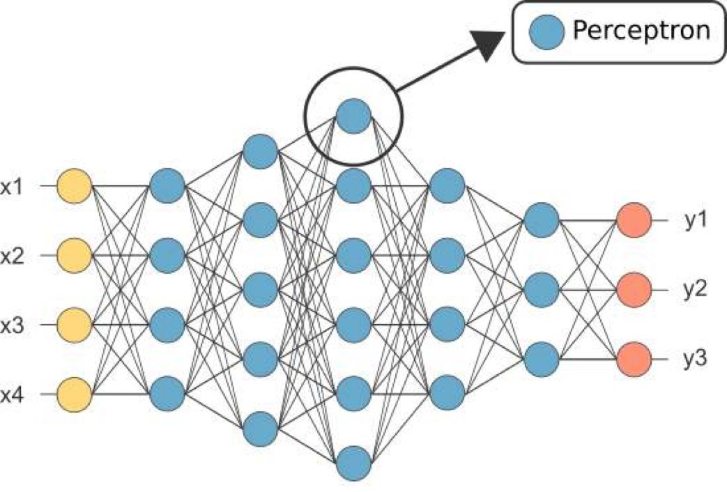
The multi-layer perceptron consists of multiple perceptrons (neurons) arranged to form a neural network. Compared to the perceptron introduced in the previous section, it adds multiple hidden layers. With the increase in the number of hidden layers, the model’s expressive power also continuously enhances, but it also increases the complexity of the network. Additionally, multi-layer perceptrons can have multiple outputs, allowing the model to be flexibly applied to multi-class tasks.
In a multi-layer perceptron, each neuron goes through an activation function, which introduces non-linear factors into the neuron, allowing the neural network to approximate any nonlinear function arbitrarily. Imagine if there were no activation functions; the output of each layer would be a linear function of the input from the previous layer. No matter how many layers the neural network has, the output would still be a linear combination of the input, rendering such a neural network meaningless.
As the number of hidden layers increases in multi-layer perceptrons, the search space for optimal weights becomes very large. Therefore, the training process of multi-layer perceptrons becomes quite complex. Generally, we use gradient descent to train the network, calculating gradients during the training process through backpropagation, which includes two stages:
-
Forward phase, where the weights of the network are fixed, and the input samples propagate forward layer by layer until the output end.
-
Backward phase, where the loss function calculates the error between the network’s output and the actual result, and the obtained error is backpropagated and derived using the chain rule to update the network’s weights via the gradient descent algorithm.
The basic flow of neural network training is as follows:
1. Given the training set, set the learning rate, and initialize all weights in the network connections;
2. Use the training set samples as network input to calculate the network output;
3. Calculate the error between the network output and the actual label using the loss function;
4. Calculate the derivative of each weight with respect to the output error using the chain rule;
5. Update each weight according to the gradient descent algorithm;
6. Repeat steps 2-5 until the convergence condition is met to finish training.
Next, we will demonstrate the forward and backward propagation processes of the multi-layer perceptron with a specific network.
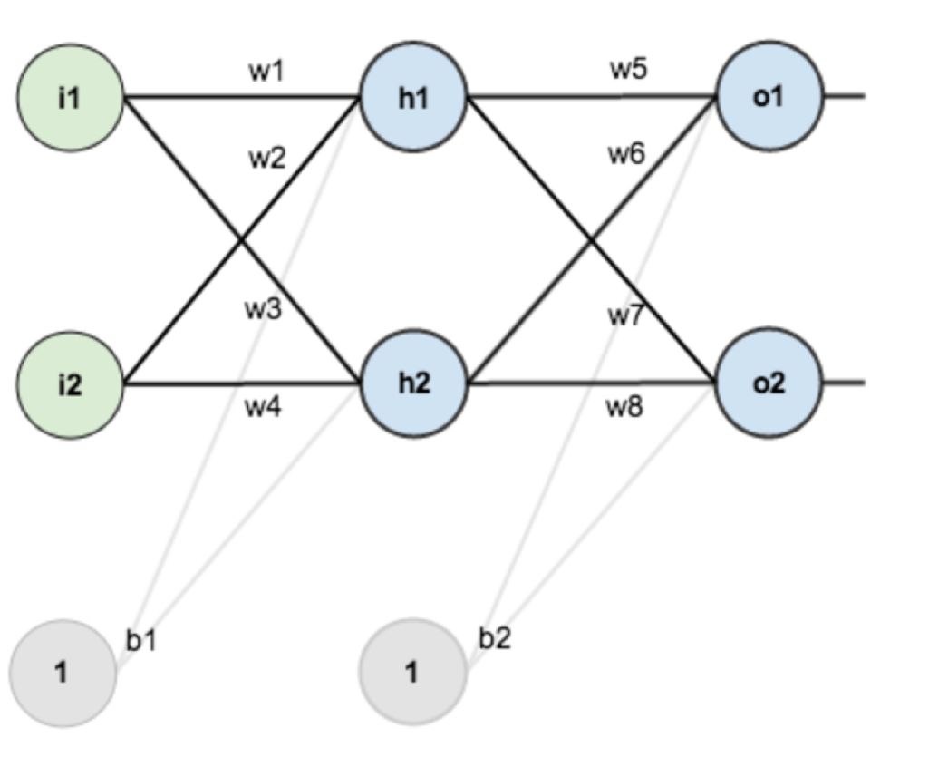
The above figure is a two-layer neural network with inputs i1 and i2, and outputs o1 and o2.
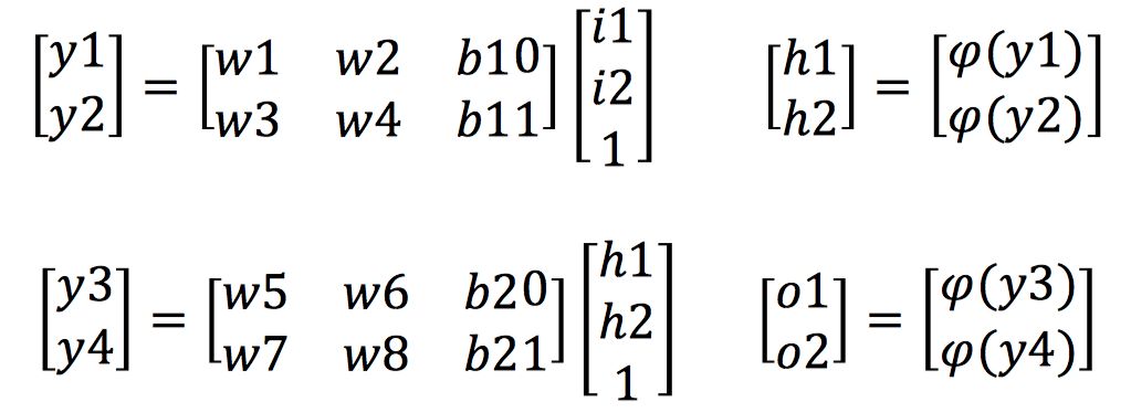
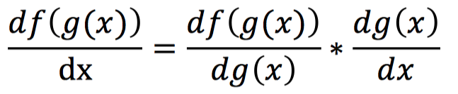
The above formula shows the calculation process of the network’s forward propagation. So what does the backpropagation process look like? Before that, let’s first introduce the core chain rule of backpropagation. The chain rule is a rule for calculating the derivative of composite functions. For a composite function f(g(x)), its derivative with respect to x can be calculated as follows:
For a composite function z=f(u,v), where u=h(x,y) and v=g(x,y), the derivatives of z with respect to x and y are calculated as follows:
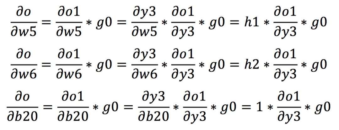
After becoming familiar with the chain rule, we start calculating the gradients of each weight in backpropagation. We assume that the gradients at the output ends o1 and o2 are g0 and g1, respectively. First, according to the chain rule, we can calculate the gradients from the output to w5, w6, and b20 as follows:

Similarly, we can further calculate the gradients from the output to other weights in the network as follows:

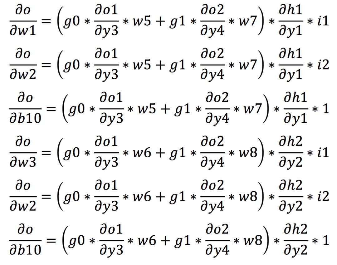
After obtaining the gradients of each weight, we further calculate the weights according to the gradient descent algorithm to achieve weight updates.
In the content introduced above, we have mentioned activation functions multiple times. The use of activation functions makes neural networks more powerful, enabling them to represent complex arbitrary function mappings between inputs and outputs non-linearly. We have already mentioned the sign activation function in the introduction to the perceptron. In this section, we will introduce three more commonly used activation functions: Sigmoid, tanh, and ReLU.
Sigmoid Activation Function, mathematically represented and corresponding to its derivative form as follows:
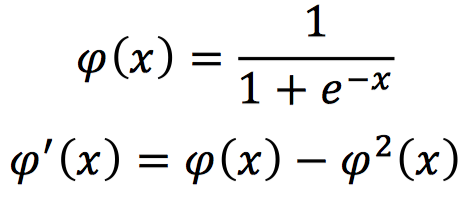
The output of this activation function is between 0 and 1. When the input is a large positive value, the output is 1; when the input is a small negative value, the output is 0.
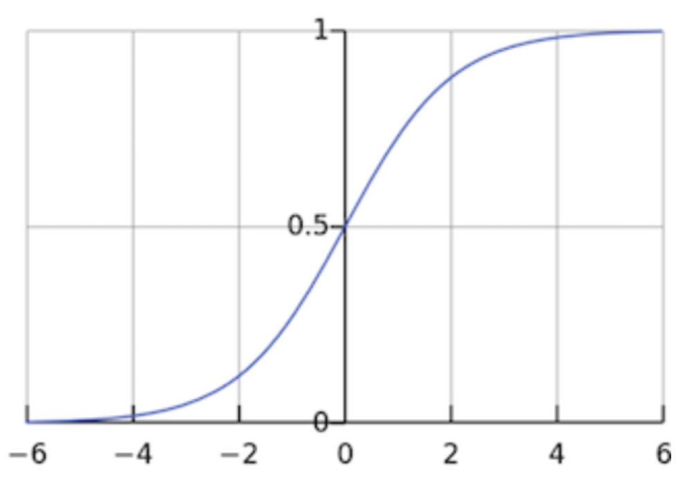
In addition, since its derivative is between 0 and 0.25, if this activation function is applied in deep neural networks, the minimum value of gradient decay during backpropagation after passing through a Sigmoid activation layer will be 0.25. When multiple Sigmoid activation functions are used, the backpropagated gradient will approach 0, which can easily lead to the vanishing gradient problem.
tanh Activation Function, mathematically represented and corresponding to its derivative form as follows:
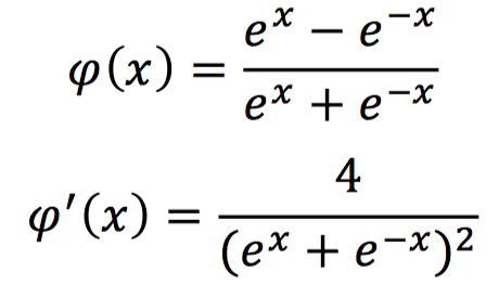
The output of this activation function is continuous between -1 and 1. When the input is a particularly large positive value, the output is 1; when the input is a small negative value, the output is -1.
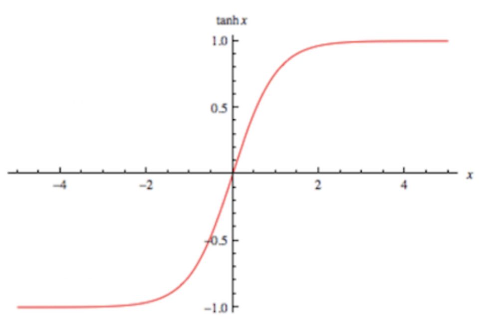
From its derivative expression, we can see that the maximum value of this activation function’s gradient is 1, distributed between 0 and 1. The further the input value deviates from 0, the smaller its gradient becomes, so there is still a vanishing gradient problem.
ReLU Activation Function, mathematically represented and corresponding to its derivative form as follows:
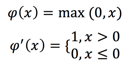
The ReLU activation function has a derivative of 1 when the input is greater than 0, which avoids the vanishing gradient problem.
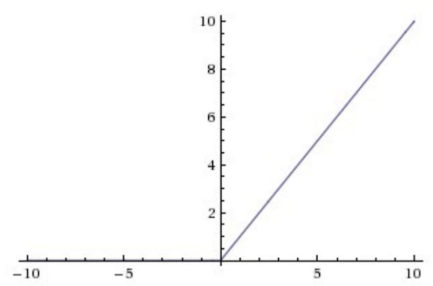
Additionally, compared to the exponential operations of Sigmoid and tanh, ReLU significantly reduces the computational load, so ReLU is now widely used in various deep neural networks. However, when the input is less than 0, its derivative is 0, and during backpropagation, there will be no gradient updates, which may cause some neurons to never activate.
The three most common activation functions are listed above. In recent years, many performance-enhanced activation functions have emerged, which we will introduce one by one in subsequent articles. In practical applications, the choice of activation functions usually relates to the performance of the network, so careful selection is necessary.
We started from basic neural networks, introducing the transition from a single perceptron to a multi-layer perceptron (MLP), from forward propagation to backpropagation, and the related content of commonly used activation functions.
In the next article, we will further transition from MLP to convolutional neural networks (CNN), and will also introduce common gradient descent optimization algorithms and loss functions. We hope that through the introduction of the basic knowledge of neural networks, everyone can better embark on a rich and colorful journey in computer vision.

Download 1: OpenCV-Contrib Extension Module Chinese Tutorial

Reply to "Extension Module Chinese Tutorial" in the "Beginner Learning Vision" public account backend to download the first Chinese version of the OpenCV extension module tutorial, covering installation of extension modules, SFM algorithms, stereo vision, object tracking, biological vision, super-resolution processing, and more than twenty chapters of content.

Download 2: Python Vision Practical Project 52 Lectures

Reply to "Python Vision Practical Project" in the "Beginner Learning Vision" public account backend to download 31 visual practical projects including image segmentation, mask detection, lane line detection, vehicle counting, eyeliner addition, license plate recognition, character recognition, emotion detection, text content extraction, and face recognition, helping to quickly learn computer vision.

Download 3: OpenCV Practical Project 20 Lectures

Reply to "OpenCV Practical Project 20 Lectures" in the "Beginner Learning Vision" public account backend to download 20 practical projects based on OpenCV, achieving advanced learning of OpenCV.

Group Chat

Welcome to join the public account reader group to exchange with peers. Currently, there are WeChat groups for SLAM, 3D vision, sensors, autonomous driving, computational photography, detection, segmentation, recognition, medical imaging, GAN, algorithm competitions, etc. (will gradually be subdivided in the future). Please scan the WeChat number below to join the group, and note: "Nickname + School/Company + Research Direction", for example: "Zhang San + Shanghai Jiao Tong University + Vision SLAM". Please follow the format for notes, otherwise, you will not be approved. After successful addition, you will be invited to relevant WeChat groups based on your research direction. Please do not send advertisements in the group, or you will be asked to leave the group, thank you for your understanding~