
Click on the above “Beginner’s Guide to Vision“, select to add “Star” or “Pin“
Important content delivered in real-time
This article is authored by Wu Yida。
https://www.cnblogs.com/wuyida/p/6301262.html
Vision-based 3D reconstruction refers to obtaining data images of scene objects through a camera, analyzing and processing these images, and then deducing the three-dimensional information of objects in the real environment by combining knowledge of computer vision.
(1) Color Images and Depth Images
Color images, also known as RGB images, have three components corresponding to the red, green, and blue channels, and their superposition forms different grayscale levels of the image pixels. The RGB color space is the foundation of the colorful real world. Depth images, also called distance images, store the distance from the pixel point to the camera instead of brightness values as in grayscale images. Figure 2-1 illustrates the relationship between depth images and grayscale images.
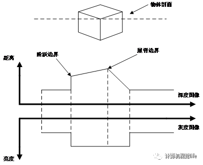 Figure 2-1 The depth image and gray image
The depth value refers to the distance between the target object and the measuring equipment. Since the depth value only relates to distance and not to environmental, lighting, or directional factors, depth images can accurately reflect the geometric depth information of scenes. By establishing a spatial model of the object, a solid foundation for deeper computer vision applications can be provided.
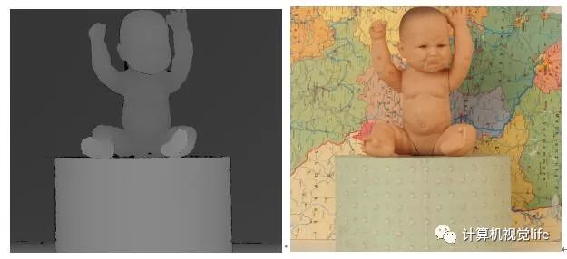 Figure 2-2 Color image and depth image of the characters
(2) PCL
PCL (Point Cloud Library) is an open-source project developed and maintained by Dr. Radu and other scholars at Stanford University based on ROS (Robot Operating System). It was initially used to assist in the development of fields such as robotic sensing, cognition, and driving. PCL was officially opened to the public in 2011. With the addition and expansion of 3D point cloud algorithms, PCL has gradually developed into a free, open-source, large-scale, cross-platform C++ programming library.
The PCL framework includes many advanced algorithms and typical data structures, such as filtering, segmentation, registration, recognition, tracking, visualization, model fitting, surface reconstruction, and many other functions. It can run on various operating systems and most embedded systems, possessing strong software portability. Given the wide application range of PCL, experts and scholars also keep the point cloud library updated and maintained in a timely manner. PCL has now reached version 1.7.0. Compared to earlier versions, it has added more fresh, practical, and interesting features, providing modular and standardized solutions for utilizing point cloud data. Moreover, through leading high-performance technologies such as graphic processors, shared storage parallel programming, and unified computing device architecture, the speed of PCL-related processes has been enhanced to achieve real-time application development.
In terms of algorithms, PCL is a set of algorithms that includes data filtering, point cloud registration, surface generation, image segmentation, and location search for processing point cloud data. Each set of algorithms is distinguished based on different types, integrating all the functions of the 3D reconstruction pipeline, ensuring the compactness, reusability, and executability of each algorithm. For example, the interface process for pipeline operations implemented in PCL is as follows:
① Create processing objects, such as filtering, feature estimation, image segmentation, etc.; ② Input initial point cloud data through setInputCloud into the processing module; ③ Set algorithm-related parameters; ④ Call functions of different functionalities to perform calculations and output results.
To achieve modular applications and development, PCL is subdivided into multiple groups of independent code collections, making it easy and quick to apply in embedded systems for portable standalone compilation. Below are some commonly used algorithm modules:
libpcl I/O: Completes the data input and output process, such as reading and writing point cloud data; libpcl filters: Completes data sampling, feature extraction, parameter fitting, etc.; libpcl register: Completes the registration process of depth images, such as the iterative closest point algorithm; libpcl surface: Completes the surface generation process of 3D models, including triangulation and surface smoothing.
These common algorithm modules all have regression testing functionality to ensure that no errors are introduced during use. Testing is generally handled by a dedicated organization that prepares the case library. When regression errors are detected, messages are immediately fed back to the corresponding authors. This enhances the safety and stability of PCL and the entire system.
(3) Point Cloud Data
As shown in Figure 2-3, it displays a typical point cloud data (PCD) model.
 Figure 2-3 Point cloud data and its magnified effect
Point cloud data typically appears in reverse engineering and is a collection of surface information of objects obtained by distance measuring devices. The scanning data is recorded in the form of points, which can be three-dimensional coordinates or information such as color or light intensity. The commonly used point cloud data generally includes point coordinate accuracy, spatial resolution, and surface normal vectors. Point clouds are generally saved in PCD format, which has strong operability and can improve the speed of point cloud registration and fusion. The point cloud data studied in this article is unstructured scattered point clouds, which are characteristic of 3D reconstruction.
(4) Coordinate Systems In three-dimensional space, all points must be represented in the form of coordinates and can be transformed between different coordinate systems. First, the concept, calculation, and interrelationship of basic coordinate systems are introduced.
① Image Coordinate System
The image coordinate system is divided into pixel and physical coordinate systems. The information of digital images is stored in matrix form, that is, the pixel image data of a picture is stored in a dimensional matrix. The image pixel coordinate system takes the origin as the reference point, using pixels as the basic unit, with U and V axes representing the horizontal and vertical directions, respectively. The image physical coordinate system takes the intersection of the camera optical axis and the image plane as the origin, using meters or millimeters as the basic unit, with its X and Y axes parallel to the U and V axes. Figure 2-4 illustrates the positional relationship between the two coordinate systems:
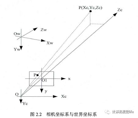 Figure 2-4 Image pixel coordinate system and physical coordinate system
Let the coordinate point (u0, v0) in the U-V coordinate system represent the physical dimensions of the pixel point on the X and Y axes. Then the relationship between all pixel points in the image in the U-V coordinate system and the X-Y coordinate system is represented by the relationship shown in formula (2-1):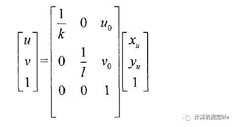
Where refers to the skew factor formed by the intersection of the coordinate axes in the image coordinate system.
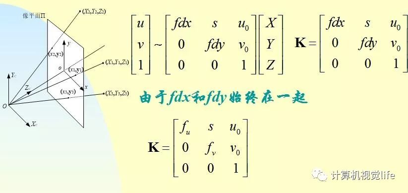
② Camera Coordinate System The camera coordinate system is composed of the optical center of the camera and three axes. Its axes correspond parallel to the axes in the physical coordinate system, and the axis is the optical axis of the camera, which is perpendicular to the plane composed of the origin and axes. As shown in Figure 2-5:
 Figure 2-5 Camera Coordinate System
Let the focal length of the camera be f, then the relationship between points in the image physical coordinate system and points in the camera coordinate system is as follows:
③ World Coordinate System
Considering the uncertainty of the camera position, it is necessary to use the world coordinate system to unify the coordinate relationship between the camera and the object. The world coordinate system consists of an origin and three axes. The transformation relationship between the world coordinate and camera coordinate is expressed by (2-3):
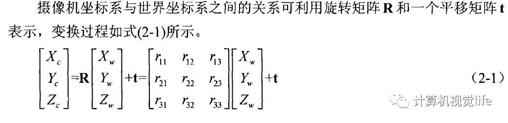


( 23 ) Where is the rotation matrix representing the camera’s orientation in the world coordinate system; is the translation vector representing the camera’s position.
This article uses Kinect to collect point cloud data of the scene, completing the 3D reconstruction of the scene through steps such as depth image enhancement, point cloud computation and registration, data fusion, and surface generation.
 Figure 2-6 Flow chart of 3D reconstruction based on depth sensor
Figure 2-6 shows that each frame of the depth image obtained undergoes the first six operations until several frames are processed. Finally, texture mapping is completed. Below is a detailed explanation of each step.
2.1 Acquisition of Depth Images
The depth images of the scene are captured by Kinect on the Windows platform, while the corresponding color images can also be obtained. To obtain a sufficient number of images, it is necessary to photograph the same scene from different angles to ensure that all information of the scene is included. The specific scheme can either fix the Kinect sensor to capture objects on a rotating platform or rotate the Kinect sensor to capture fixed objects. Affordable and easy-to-operate depth sensor devices can acquire real-time depth images of scenes, greatly facilitating applications.
2.2 Preprocessing
Due to limitations such as device resolution, its depth information has many drawbacks. To better facilitate subsequent applications based on depth images, the depth images must undergo denoising and enhancement processes. The specific processing methods will be explained in detail in Chapter Four, as this is a key issue in this article.
2.3 Point Cloud Computation
After preprocessing, the depth images possess two-dimensional information, where the pixel values represent depth information, indicating the straight-line distance from the object surface to the Kinect sensor, measured in millimeters. Based on the principle of camera imaging, the transformation relationship between the world coordinate system and the image pixel coordinate system can be calculated as follows:
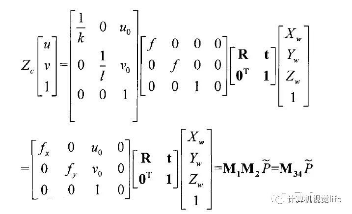
Thus, k value only relates to , while parameters only relate to the internal structure of the camera, hence referred to as the camera’s intrinsic parameter matrix. Taking the camera as the world coordinate system, the depth value corresponds to the value in the world coordinate system, and the corresponding image coordinate is the point on the image plane.
2.4 Point Cloud Registration
For multiple frames of images captured from different angles, each frame contains a certain common part. To utilize depth images for 3D reconstruction, it is necessary to analyze the images and solve the transformation parameters between frames. The registration of depth images is based on the common parts of the scene, overlaying multiple frames of images obtained at different times, angles, and lighting conditions into a unified coordinate system. The corresponding translation vector and rotation matrix are computed, while redundant information is eliminated. Point cloud registration not only affects the speed of 3D reconstruction but also influences the fineness and global effect of the final model. Thus, it is crucial to improve the performance of point cloud registration algorithms.
The registration of three-dimensional depth information is categorized into three methods based on different image input conditions and reconstruction output requirements: coarse registration, fine registration, and global registration.
(1) Coarse Registration
Coarse registration studies depth images collected from multiple frames at different angles. First, feature points between two frames of images are extracted; these feature points can be explicit features such as lines, corners, curve curvatures, or custom symbols, rotated shapes, and axes.
Then, preliminary registration is achieved based on feature equations. The point cloud after coarse registration and the target point cloud will be at the same scale (pixel sampling interval) within the reference coordinate system, obtaining coarse matching initial values through automatic coordinate recording.
(2) Fine Registration
Fine registration is a deeper registration method. After the previous coarse registration, a transformation estimate is obtained. This value is used as the initial value, and through continuous convergence and iterative fine registration, a more precise effect is achieved. Taking the classic ICP (Iterative Closest Point) algorithm proposed by Besl and Mckay as an example, this algorithm first calculates the distance between all points on the initial point cloud and the target point cloud, ensuring that these points correspond to the nearest points of the target point cloud while constructing a target function of the residual sum of squares.
Based on the least squares method, the error function is minimized through repeated iterations until the mean square error is below a set threshold. The ICP algorithm can achieve accurate registration results, which is significant for the registration problem of free-form surfaces. Other algorithms such as SAA (Simulated Annealing Algorithm) and GA (Genetic Algorithm) also have their characteristics and usage domains.
(3) Global Registration
Global registration uses the entire image to directly compute the transformation matrix. Through the fine registration results of two frames, multiple frames of images are registered in a certain sequence or all at once. These two registration methods are called sequential registration and simultaneous registration, respectively.
During the registration process, matching errors are evenly distributed across multiple frames of images from various perspectives, reducing the cumulative errors caused by multiple iterations. It is worth noting that, although global registration can reduce errors, it consumes a large amount of memory storage space and significantly increases the time complexity of the algorithm.
2.5 Data Fusion
After registration, the depth information remains as scattered unordered point cloud data in space, only exhibiting partial information of the scene. Therefore, point cloud data must undergo fusion processing to obtain a more refined reconstruction model. A volumetric grid is constructed with the initial position of the Kinect sensor as the origin, dividing the point cloud space into numerous small cubes, called voxels. By assigning SDF (Signed Distance Field) values to all voxels, the surface is implicitly simulated.
The SDF value equals the minimum distance from this voxel to the reconstructed surface. When the SDF value is greater than zero, it indicates that the voxel is in front of the surface; when the SDF is less than zero, it indicates that the voxel is behind the surface; the closer the SDF value is to zero, the closer the voxel is to the actual surface of the scene. Although KinectFusion technology has efficient real-time performance for scene reconstruction, its reconstructable spatial range is limited, mainly due to the large amount of space consumed to store numerous voxels.
To address the issue of voxel occupying a large amount of space, Curless and others proposed the TSDF (Truncated Signed Distance Field) algorithm, which only stores a few layers of voxels that are close to the actual surface, rather than all voxels. This significantly reduces the memory consumption of KinectFusion and minimizes model redundancy.
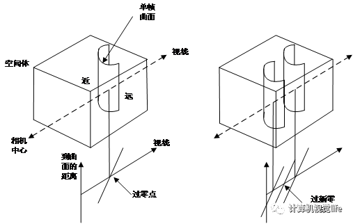 Figure 2-7 Point cloud fusion based on spatial volume
The TSDF algorithm uses grid cubes to represent three-dimensional space, with each grid storing its distance to the object surface. The positive and negative values of the TSDF indicate the occluded and visible surfaces, respectively, while points on the surface pass through the zero point. As shown on the left side of Figure 2-7, it displays a model within a grid cube. If another model enters the cube, fusion processing is performed according to formulas (2-9) and (2-10).
Where refers to the distance from the point cloud to the grid at this time, is the initial distance of the grid, and is the weight used to fuse the distance values of the same grid. As shown on the right side of Figure 2-7, the sum of the two weights is the new weight. For the KinectFusion algorithm, the weight value of the current point cloud is set to 1.
Given that the TSDF algorithm is optimized using the least squares method and utilizes weight values during point cloud fusion, this algorithm exhibits significant denoising capabilities for point cloud data.
2.6 Surface Generation
The purpose of surface generation is to construct the visible isosurface of an object, commonly using voxel-level methods to directly process the original grayscale volumetric data.Lorensen proposed the classic voxel-level reconstruction algorithm: MC (Marching Cubes) method.The marching cubes method first stores the data from eight adjacent positions in a tetrahedral volume element at the eight vertices.For an edge of a boundary voxel with two endpoints, when one value is greater than a given constant T and the other is less than T, then there must be a vertex of the isosurface on that edge.
Then, the intersection points of the twelve edges in the volume element and the isosurface are calculated, and triangular patches are constructed within the volume element, dividing the element into regions inside and outside the isosurface. Finally, connecting all triangular patches from the data field of this volume element forms the isosurface. Merging all isosurfaces of the cubes generates a complete 3D surface.
The advent of depth sensors such as Kinect has not only transformed entertainment applications but also provided new directions for scientific research, especially in the field of 3D reconstruction. However, since the 3D reconstruction process involves processing a large amount of dense point cloud data, which requires significant computational power, optimizing the system’s performance becomes very important. This article adopts GPU (Graphic Processing Unit) parallel computing capabilities to enhance overall operational efficiency.
NVIDIA introduced the concept of GPU in 1999. Over the past decade, with innovations in the hardware industry, the number of transistors on chips has continuously increased, and GPU performance has doubled every six months. The floating-point computing power of GPUs far exceeds that of CPUs by hundreds of times, while having very low energy consumption, making it highly cost-effective. GPUs are not only widely used in graphics and image processing but have also emerged in fields such as video processing, oil exploration, biochemistry, satellite remote sensing data analysis, weather forecasting, and data mining.
As the proponent of GPUs, NVIDIA has been dedicated to researching GPU performance enhancement and launched the CUDA architecture in 2007. CUDA (Compute Unified Device Architecture) is a parallel computing programming architecture. With the support of CUDA, users can write programs to utilize NVIDIA series GPUs for large-scale parallel computing. In CUDA, the computer CPU is referred to as the host, while the GPU is referred to as the device.
Both the host and device run programs, with the host primarily completing the program flow and serial computation modules, while the device specifically handles parallel computations. The parallel computation process on the device is recorded in Kernel functions, which the host can invoke to execute parallel computation calls from the Kernel function entry. During this process, although the Kernel function executes the same code, it processes different data content.
The Kernel function is programmed using an extended C language, known as CUDAC language. It is important to note that not all computations can be performed using CUDA parallel computing. Only independent calculations, such as matrix addition and subtraction, can be parallelized, as they only involve the addition and subtraction of elements with corresponding indices, and elements with different indices are unrelated. However, calculations like factorial must accumulate all numbers multiplicatively, and thus cannot be parallelized.
CUDA has a three-level architecture of threads, blocks, and grids, where the computation process is generally completed by a single grid, which is evenly divided into multiple blocks, with each block consisting of multiple threads, and finally a single thread completes each basic computation, as shown in Figure 2-8.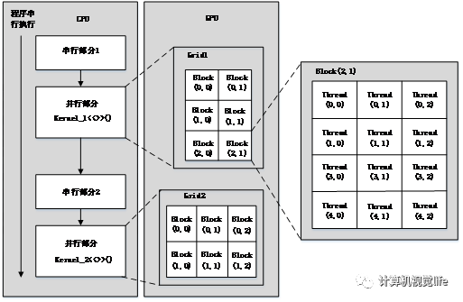 Figure 2-8 CUDA model
To gain a deeper understanding of the CUDA model’s computation process, the formula (2-11) mentioned in the previous chapter is taken as an example to calculate the transformation between the depth value of a certain point and its three-dimensional coordinates: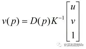 The depth value in the formula represents the depth value, and the intrinsic parameter matrix is a known quantity, which is the coordinates of that point. It can be observed that the transformation process of this point is independent of other points, so the coordinate transformations of each point in the entire image can be executed in parallel. This parallel computation can significantly enhance the overall computation speed. For instance, using a grid to compute the transformation of a pixel’s depth image to three-dimensional coordinates only requires dividing this grid into blocks, with each block containing threads, and each thread operating on a pixel point, thus easily completing all coordinate transformation calculations.
Through parallel computing with GPUs, the performance of 3D reconstruction has been significantly improved, achieving real-time input and output, laying the foundation for the application of Kinect in practical production and life.
First, the basic concepts related to 3D reconstruction, including depth images, point cloud data, four coordinate systems, and their transformation relationships, are introduced.
Good news!
Beginner’s Guide to Vision Knowledge Planet
Is now open to the public 👇👇👇
Download 1: Chinese Tutorial for OpenCV-Contrib Extension Modules

Reply "Chinese Tutorial for Extension Modules" in the background of "Beginner's Guide to Vision" public account to download the first Chinese version of the OpenCV extension module tutorial on the internet, covering installation of extension modules, SFM algorithms, stereo vision, target tracking, biological vision, super-resolution processing, and more than twenty chapters of content.

Download 2: 52 Lectures on Practical Python Vision Projects

Reply "Python Vision Practical Projects" in the background of "Beginner's Guide to Vision" public account to download 31 practical vision projects including image segmentation, mask detection, lane line detection, vehicle counting, eyeliner addition, license plate recognition, character recognition, emotion detection, text content extraction, facial recognition, etc., to help quickly learn computer vision.

Download 3: 20 Lectures on Practical OpenCV Projects

Reply "20 Lectures on Practical OpenCV Projects" in the background of "Beginner's Guide to Vision" public account to download 20 practical projects based on OpenCV for advanced learning of OpenCV.

Group Chat

Welcome to join the public account reader group to communicate with peers. Currently, there are WeChat groups for SLAM, 3D vision, sensors, autonomous driving, computational photography, detection, segmentation, recognition, medical imaging, GAN, algorithm competitions, etc. (these will gradually be subdivided). Please scan the WeChat ID below to join the group, and note: "Nickname + School/Company + Research Direction", for example: "Zhang San + Shanghai Jiao Tong University + Vision SLAM". Please follow the format for remarks, otherwise, you will not be approved. After successful addition, invitations to related WeChat groups will be sent based on research direction. Please do not send advertisements in the group, or you will be removed from the group. Thank you for your understanding~