1. Linear Regression
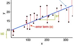
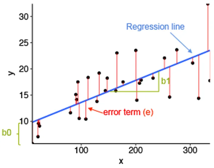
Linear regression is a statistical method used to study the relationship between two continuous variables: one independent variable and one dependent variable. The goal of linear regression is to find the best-fit line through a set of data points, which can then be used to predict future observations.
The equation for a simple linear regression model is:
y = b0 + b1*x
where y is the dependent variable, x is the independent variable, b0 is the intercept (the point where the line intersects the y-axis), and b1 is the slope of the line. The slope indicates the change in y given a change in x.
To determine the best-fit line, we use the least squares method to find the line that minimizes the sum of the squared differences between the predicted and actual values.
Linear regression can also be extended to multiple independent variables, known as multiple linear regression. The equation for the multiple linear regression model is:
y = b0 + b1x1 + b2x2 + … + bn*xn
where x1, x2, …, xn are the independent variables, and b1, b2, …, bn are the corresponding coefficients.
Linear regression can be used for both simple linear regression and multiple linear regression problems. The coefficients b0 and b1, …, bn are estimated using the least squares method. Once the coefficients are estimated, they can be used to predict the dependent variable.
Linear regression can be used to predict future scenarios, such as forecasting stock prices or product sales. However, linear regression is a relatively simple method and is not suitable for all problems. It assumes that the relationship between the independent and dependent variables is linear, which is not always the case.
Additionally, linear regression is very sensitive to outliers, meaning that if there are any extreme values that do not follow the overall trend of the data, they can significantly affect the model’s accuracy.
In summary, linear regression is a powerful and widely used statistical method for studying the relationship between two continuous variables. It is a simple yet powerful tool for making predictions about the future. However, keep in mind that linear regression assumes a linear relationship between variables and is very sensitive to outliers, which can affect the model’s accuracy.
2. Logistic Regression
Logistic regression is a statistical method used to predict a binary outcome based on one or more independent variables, such as success or failure. It is a popular technique in machine learning and is often used for classification tasks, such as determining whether an email is spam or predicting whether a customer will churn.
The logistic regression model is based on the logistic function, which is an S-shaped function that maps input variables to probabilities between 0 and 1. This probability is then used to make predictions about the outcome.
The logistic regression model is represented by the following equation:
P(y=1|x) = 1/(1+e^-(b0 + b1x1 + b2x2 + … + bn*xn))
where P(y=1|x) is the probability that the outcome y is 1 given the input variables x, b0 is the intercept, and b1, b2, …, bn are the coefficients for the input variables x1, x2, …, xn.
These coefficients are determined by training the model on a dataset and using optimization algorithms (such as gradient descent) to minimize the cost function (usually the log loss).
Once the model is trained, predictions can be made by inputting new data and calculating the probability of the outcome being 1. The threshold for classifying the result as 1 or 0 is typically set around 0.5, but this depends on the specific task and the trade-off between false positives and false negatives.
Here is a chart representing the logistic regression model:
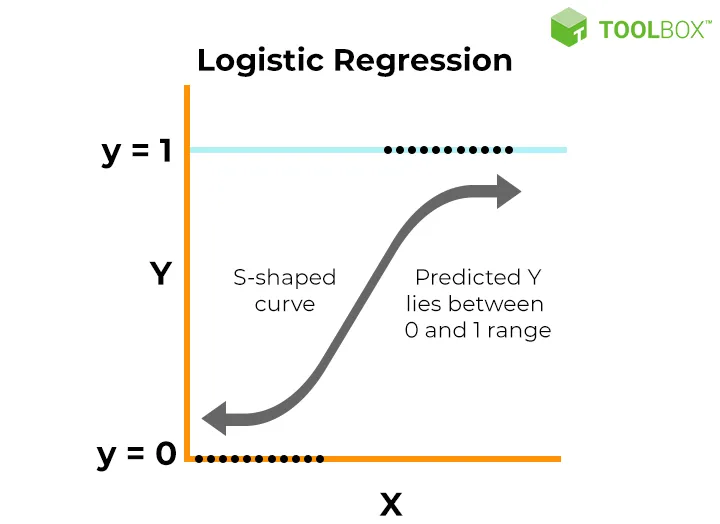
In this chart, the input variables x1 and x2 are used to predict the binary outcome y. The logistic function maps the input variables to probabilities, which are then used to make predictions. The coefficients b1 and b2 are determined by training the model on the dataset, and the threshold is set at 0.5.
In summary, logistic regression is a powerful technique for predicting binary outcomes, widely used in machine learning and data analysis. It is easy to implement, interpret, and can be easily regularized to prevent overfitting.
3. Support Vector Machines
Support Vector Machines (SVM) are a type of supervised learning algorithm that can be used for classification or regression problems. The main idea of SVM is to find the boundary that separates different classes in the data by maximizing the margin, which is the distance between the boundary and the nearest data points of each class. These nearest data points are called support vectors.
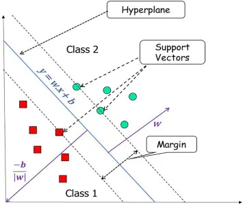
SVM is particularly useful when the data is not linearly separable, meaning it cannot be separated by a straight line. In these cases, SVM can use a technique called the kernel trick to transform the data into a higher-dimensional space where a non-linear boundary can be found. Some common kernel functions used in SVM include polynomial, radial basis function (RBF), and sigmoid.
One of the main advantages of SVM is that they are very effective in high-dimensional spaces and perform well even when the number of features exceeds the number of samples. Additionally, SVM is memory efficient because it only needs to store the support vectors rather than the entire dataset.
On the other hand, SVM can be sensitive to the choice of kernel function and algorithm parameters. It is also important to note that SVM may not be suitable for large datasets due to potentially long training times.
Advantages:
-
Effective in high-dimensional spaces: SVM performs well even when the number of features exceeds the number of samples.
-
Memory efficient: SVM only needs to store support vectors rather than the entire dataset, making it memory efficient.
-
Versatile: SVM can be used for both classification and regression problems and can handle non-linearly separable data using the kernel trick.
-
Robust to noise and outliers: Since it only relies on support vectors, SVM is robust to noise and outliers in the data.
Disadvantages:
-
Sensitive to kernel function and parameter selection: The performance of SVM can be significantly affected by the choice of kernel function and algorithm parameters.
-
Not suitable for large datasets: Training SVM on large datasets can be time-consuming.
-
Difficult to interpret results: Especially when using non-linear kernels, interpreting SVM results can be challenging.
-
Struggles with overlapping classes: SVM may not perform well when classes have significant overlap.
In summary, Support Vector Machines (SVM) are powerful supervised learning algorithms that can be used for both classification and regression problems, particularly when the data is not linearly separable. This algorithm is known for its good performance in high-dimensional spaces and its ability to find non-linear boundaries. However, it is sensitive to the choice of kernel function and parameters and is not suitable for large datasets.
4. Decision Trees
Decision trees are a type of machine learning algorithm used for classification and regression tasks. They are powerful tools for decision-making and can model complex relationships between variables.
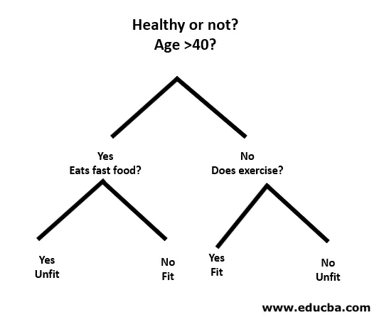
A decision tree is a model that resembles a tree structure, where each internal node represents a decision point and each leaf node represents an outcome or prediction. The tree is constructed by recursively splitting the data into subsets based on input feature values. The goal is to find the splits that maximize the separation between different classes or target values.
One of the main advantages of decision trees is that they are easy to understand and interpret. The tree structure allows for clear visualization of the decision-making process, and the importance of each feature can be easily assessed.
The process of building a decision tree begins with selecting the root node, which is the feature that best separates the data into different classes or target values. The data is then split into subsets based on the values of that feature, and this process is repeated for each subset until a stopping criterion is met. Stopping criteria can be determined based on factors such as the number of samples in the subset, purity, or tree depth.
One of the main disadvantages of decision trees is that they are prone to overfitting, especially when the tree is deep and has many leaf nodes. Overfitting occurs when the decision tree becomes too complex and fits the noise in the data rather than the underlying patterns. This can lead to poor performance on unseen data. To prevent overfitting, techniques such as pruning, regularization, and cross-validation can be used.
Another issue is that decision trees are sensitive to the order of input features. Different orders of features can lead to different tree structures, and the final outcome may not be optimal. To overcome this issue, techniques such as random forests and gradient boosting have been developed.
In summary, decision trees are a powerful and versatile tool for decision-making and predictive modeling. They are easy to understand and interpret, but they are prone to overfitting. Various techniques have been developed to overcome these limitations, such as pruning, regularization, cross-validation, random forests, and gradient boosting.
Advantages:
-
Easy to understand and interpret: The tree structure allows for clear visualization of the decision-making process, and the importance of each feature can be easily assessed.
-
Handles numerical and categorical data: Decision trees can handle both numerical and categorical data, making them a versatile tool widely used.
-
High accuracy: Decision trees can achieve high accuracy on many datasets, especially when the tree is not deep.
-
Robust to outliers: Decision trees are not affected by outliers and are well-suited for datasets with noise.
-
Can be used for classification and regression tasks.
Disadvantages:
-
Overfitting: Decision trees are prone to overfitting, especially when the tree is deep and has many leaf nodes.
-
Sensitive to the order of input features: Different orders of features can lead to different tree structures, and the final outcome may not be optimal.
-
Unstable: Decision trees are sensitive to small changes in the data, which can lead to different tree structures and prediction outcomes.
-
Bias: Decision trees may be biased towards features with more levels or categorical variables with many levels, leading to inaccurate predictions.
-
Poor performance with continuous variables: Decision trees may perform poorly if the variable is continuous. If the variable is divided into many levels, it can make the decision tree complex and lead to overfitting.
5. Random Forests
Random forests are an ensemble machine learning algorithm used for classification and regression tasks. It is a combination of multiple decision trees, where each tree is grown using a random subset of the data and a random subset of features. The final prediction is achieved by averaging the predictions of all trees in the forest.
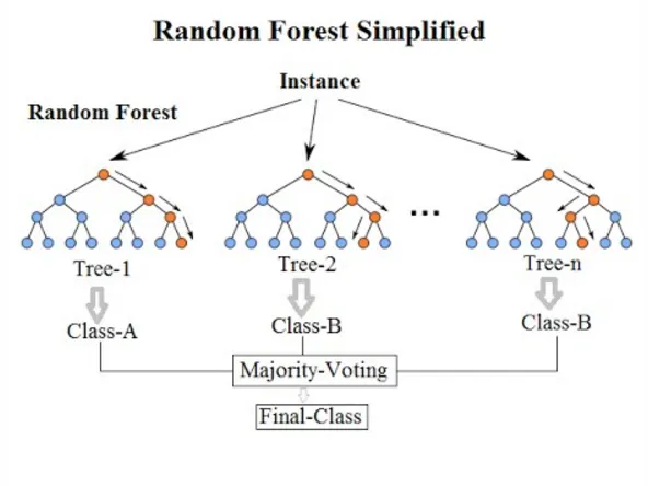
The idea of using multiple decision trees is that while a single decision tree may easily overfit, an ensemble of decision trees, or a forest, can reduce the risk of overfitting and improve the overall accuracy of the model.
The process of building a random forest begins with creating multiple decision trees using a technique called bootstrapping. Bootstrapping is a statistical method that involves randomly selecting data points from the original dataset with replacement. This creates multiple datasets, each with different data points, which are then used to train individual decision trees.
Another important aspect of random forests is using a random subset of features for each tree. This is known as the random subspace method. This reduces the correlation between trees in the forest, thereby improving the overall performance of the model.
One of the main advantages of random forests is that they are less prone to overfitting compared to a single decision tree. The averaging of multiple trees can smooth out errors and reduce variance. Random forests also perform well on high-dimensional datasets and datasets with a large number of categorical variables.
The downside of random forests is that they have high computational costs for training and prediction. As the number of trees in the forest increases, the computational time also increases. Additionally, the interpretability of random forests is poorer than that of a single decision tree because it is more difficult to understand the contribution of each feature to the final prediction.
In summary, random forests are a powerful ensemble machine learning algorithm that can improve the accuracy of decision trees. They are less prone to overfitting and perform well on high-dimensional and categorical datasets. However, they have high computational costs and are less interpretable than a single decision tree.
Due to space limitations, this is the first half of the introduction, and the remaining algorithms will be continued in the next article.

Author:Ji Suan Simulation
Selected by: Wang Huajun
Edited by: Liu Yimei