

Selected from TowardsDataScience
Author: Kerem Turgutlu
Translation by: Machine Heart
Contributors: Panda
This article is reprinted from the “Machine Heart” WeChat official account
This blog mainly focuses on a lesser-known application area in the field of deep learning: structured data. The author of this article is Kerem Turgutlu, a graduate student at the University of San Francisco (USF).
The benefits of using deep learning methods to process structured data as described in this article include:
-
Fast
-
No domain knowledge required
-
Excellent performance
In any machine learning/deep learning or any type of predictive modeling task, data is first available, and then algorithms/methods are applied. This is also the main reason why certain machine learning methods require extensive feature engineering before solving specific tasks, including image classification, NLP, and many other “unconventional” data processing tasks—data that cannot be directly fed into logistic regression or random forest models. In contrast, deep learning can achieve good performance on these types of tasks without any complicated and time-consuming feature engineering. Most of the time, these features require domain knowledge, creativity, and a lot of trial and error. Of course, domain expertise and sophisticated feature engineering are still very valuable, but the techniques mentioned in this article are sufficient to help you compete for a top-three position in Kaggle competitions without any domain knowledge, see: http://blog.kaggle.com/2016/01/22/rossmann-store-sales-winners-interview-3rd-place-cheng-gui/

Figure 1: A cute dog and an angry cat
Due to the complex nature and capacity of feature generation (e.g., convolutional layers of CNN), deep learning has found widespread applications in various image, text, and audio data problems. These issues are undoubtedly crucial for the development of artificial intelligence, and top researchers in this field are competing annually on tasks such as classifying cats, dogs, and ships, with each year’s results surpassing the previous year. However, we rarely see this situation in practical industry applications. Why is that? The databases of companies involve structured data, which are the domains that shape our daily lives.
First, let’s define structured data. In structured data, you can think of rows as the collected data points or observations and columns as fields representing individual attributes of each observation. For example, data from an online retail store has columns representing customer transaction events and columns containing information about purchased items, quantities, prices, timestamps, etc.
Below, we provide some seller data, where rows represent each independent sales event, and columns provide information about these sales events.

Figure 2: Example of structured data in a pandas dataframe
Next, let’s discuss how to use neural networks for structured data tasks. In theory, it is quite simple to create a fully connected network with any desired architecture and then use the “columns” as input. After the loss function undergoes some dot products and backpropagation, we will obtain a trained network that can then make predictions.
Although it seems very straightforward, people often prefer tree-based methods over neural networks when dealing with structured data. Why is that? This can be understood from the perspective of algorithms—how the algorithms treat and process our data.
People handle structured and unstructured data differently. While unstructured data is “unconventional”, we typically deal with single entities of unit quantities, such as pixels, voxels, audio frequencies, radar backscatter, sensor measurements, etc. For structured data, we often need to handle various types of data; these data types fall into two main categories: numerical data and categorical data. Categorical data needs preprocessing before training because most algorithms, including neural networks, cannot directly handle them.
There are many optional methods for encoding variables, such as label/numeric encoding and one-hot encoding. However, these techniques still have issues regarding memory and the true representation of categorical hierarchies. Memory issues may be more pronounced, which we will illustrate with an example.
Assuming the information in our column is a day of the week. If we use one-hot or any label encoding for this variable, we must assume that there are equal and arbitrary distances/differences between each level.
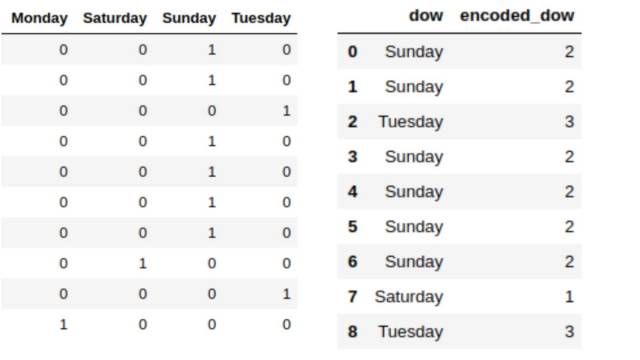
Figure 3: One-hot encoding and label encoding
But both methods assume that the difference between any two days is equal, which we clearly know is not the case, and our algorithms should recognize that!
“The continuity nature of neural networks limits their application on categorical variables. Therefore, using integer numbers to represent categorical variables and then directly applying neural networks does not yield good results.”[1]
Tree-based algorithms do not require the assumption that categorical variables are continuous, as they can branch as needed to find each state, but neural networks cannot do that. Entity embeddings can help solve this problem. Entity embeddings can be used to map discrete values into a multidimensional space, where values with similar functional outputs are closer to each other. For example, if you want to embed various provinces into the national space for a sales problem, then similar provinces’ sales will be closer in this projected space.
Since we do not want to make any assumptions about the hierarchy of our categorical variables, we will learn a better representation of each category in Euclidean space. This representation is simple and is equivalent to the dot product of one-hot encoding with learnable weights.
Embeddings have widespread applications in the NLP field, where each word can be represented as a vector. Glove and word2vec are two famous embedding methods. We can see the power of embeddings from Figure 4 [2]. As long as these vectors fit your goals, you can download and use them anytime; this is indeed a good way to represent the information they contain.
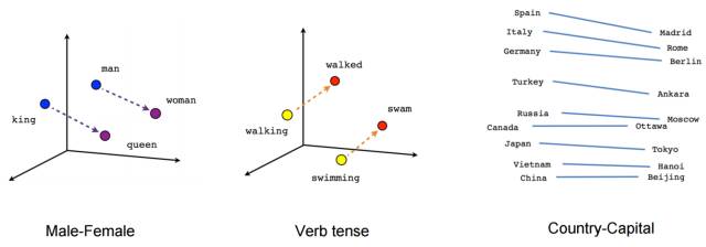
Figure 4: word2vec from TensorFlow tutorial
Although embeddings can be used in different contexts (whether supervised or unsupervised methods), our main goal is to understand how to perform this mapping for categorical variables.
Entity Embeddings
Although people have different interpretations of “entity embeddings”, they are not significantly different from the use cases we see in word embeddings. After all, we only care that our grouped data has a higher-dimensional vector representation; this data may be words, days of the week, countries, etc. This transformation from word embeddings to metadata embeddings (in our case, categories) was used by Yoshua Bengio et al. to win a Kaggle competition in 2015 using a simple automated method—something that typically would not win competitions. See: https://www.kaggle.com/c/pkdd-15-predict-taxi-service-trajectory-i
“To handle discrete metadata consisting of customer IDs, taxi IDs, date, and time information, we used the model to jointly learn embeddings for each of these pieces of information. This approach was inspired by natural language modeling methods [2], where each word is mapped to a fixed-size vector space (this vector is called a word embedding). [3]
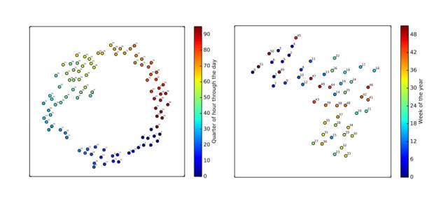
Figure 5: Visualization of taxi metadata embeddings obtained using t-SNE 2D projection
We will explore step by step how to learn these features in a neural network. Define a fully connected neural network and then handle numerical and categorical variables separately.
For each categorical variable:
1. Initialize a random embedding matrix mxD:
m: number of different levels of categorical variables (Monday, Tuesday, etc.)
D: the desired dimension for representation, which is a hyperparameter that can take values from 1 to m-1 (1 means label encoding, m means one-hot encoding)
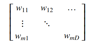
Figure 6: Embedding matrix
2. Then, for each forward pass in the neural network, we query the given label (e.g., querying Monday for “dow”) in the embedding matrix, which will yield a 1xD vector.
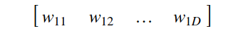
Figure 7: Retrieved embedding vector
3. Append this 1×D vector to our input vector (numerical vector). You can think of this process as matrix augmentation, where we add an embedding vector for each category, obtained by performing a lookup for each specific row.
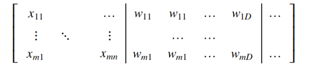
Figure 8: After adding the embedding vector
4. While performing backpropagation, we also update these embedding vectors in a gradient manner to minimize our loss function.
Inputs generally do not get updated, but there is a special case for the embedding matrix where we allow our gradient to flow back through these mapped features to optimize them.
We can think of it as a process that allows categorical embeddings to represent better after each iteration.
Note: Empirically, categories without very high cardinality should be retained. Because if a specific level of a variable accounts for 90% of observations, then it is a variable with poor predictive value, and we may as well avoid it.
Good News
By performing lookups in our embedding vectors and allowing requires_grad=True and learning them, we can effectively implement the architecture mentioned above in our favorite frameworks (preferably dynamic frameworks). However, Fast.ai has already implemented all these steps and done more. Besides making structured deep learning easier, this library also provides many state-of-the-art features, such as differential learning rates, SGDR, cyclical learning rates, learning rate finder, etc. These are all features we can take advantage of. You can learn more about these topics in the following blogs:
https://medium.com/@bushaev/improving-the-way-we-work-with-learning-rate-5e99554f163b
https://medium.com/@surmenok/estimating-optimal-learning-rate-for-a-deep-neural-network-ce32f2556ce0
https://medium.com/@markkhoffmann/exploring-stochastic-gradient-descent-with-restarts-sgdr-fa206c38a74e
Implementing with Fast.ai
In this section, we will introduce how to implement the above steps and build a neural network that can handle structured data more effectively.
To do this, let’s look at a popular Kaggle competition: https://www.kaggle.com/c/mercari-price-suggestion-challenge/. This is a very suitable example for entity embeddings because its data is mostly categorical and has a relatively high cardinality (but not too high), and there isn’t much else.
Data:
About 1.4 million rows
-
item_condition_id: Condition of the item (cardinality: 5)
-
category_name: Category name (cardinality: 1287)
-
brand_name: Brand name (cardinality: 4809)
-
shipping: Whether the price includes shipping (cardinality: 2)
Important Note: Since I have found the best model parameters, I will not include a validation set in this example, but you should use a validation set to tune hyperparameters.
Step 1:
Treat missing values as a separate level, as missingness itself is also important information.
train.category_name = train.category_name.fillna('missing').astype('category')
train.brand_name = train.brand_name.fillna('missing').astype('category')
train.item_condition_id = train.item_condition_id.astype('category')
test.category_name = test.category_name.fillna('missing').astype('category')
test.brand_name = test.brand_name.fillna('missing').astype('category')
test.item_condition_id = test.item_condition_id.astype('category')
Step 2:
Preprocess the data, scaling numerical columns proportionally, since neural networks prefer normalized data. If you do not scale your data, the network may place extra emphasis on one feature, as it is all just dot products and gradients. It would be better if we scale both training and testing data based on training statistics, but this should not have a significant impact. It’s similar to dividing each pixel’s value by 255.
Since we want the same levels to have the same encoding, I combined the training and testing data.
combined_x, combined_y, nas, _ = proc_df(combined, 'price', do_scale=True)Step 3:
Create a model data object. The path is where Fast.ai stores models and activations.
path = '../data/'
md = ColumnarModelData.from_data_frame(path, test_idx, combined_x, combined_y, cat_flds=cats, bs=128)
Step 4:
Determine D (the dimension of the embedding), cat_sz is a list of tuples (col_name, cardinality+1) for each categorical column.
# We said that D (dimension of embedding) is a hyperparameter
# But here is Jeremy Howard's rule of thumb
emb_szs = [(c, min(50, (c+1)//2)) for _,c in cat_sz]
# [(6, 3), (1312, 50), (5291, 50), (3, 2)]
Step 5:
Create a learner, which is the core object of the Fast.ai library.
params: embedding sizes, number of numerical cols, embedding dropout, output, layer sizes, layer dropouts
m = md.get_learner(emb_szs, len(combined_x.columns)-len(cats),
                   0.04, 1, [1000,500], [0.001,0.01], y_range=y_range)
Step 6:
This part is explained in more detail in other articles I mentioned earlier.
To fully leverage Fast.ai’s advantages.
At some point before the loss starts to increase, we need to choose our learning rate……
# find best lr
m.lr_find()
# find best lr
m.sched.plot()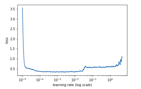
Figure 9: Learning rate vs loss graph
Fitting
We can see that after just 3 epochs, we get:
lr = 0.0001
m.fit(lr, 3, metrics=[lrmse])
More Fitting
m.fit(lr, 3, metrics=[lrmse], cycle_len=1)
And More……
m.fit(lr, 2, metrics=[lrmse], cycle_len=1)
So, in just a few minutes, without further operations, these simple yet effective steps can place you in about the top 10%. If you really have higher goals, I recommend using the item_description column and treating it as multiple categorical variables. Then let entity embeddings do the work, and of course, don’t forget to stack and combine.
References
[1] Cheng Guo, Felix Berkhahn (2016, April, 22) Entity Embeddings of Categorical Variables. Retrieved from https://arxiv.org/abs/1604.06737.
[2] TensorFlow Tutorials: https://www.tensorflow.org/tutorials/word2vec
[3] Yoshua Bengio, et al. Artificial Neural Networks Applied to Taxi Destination Prediction. Retrieved from* **https://arxiv.org/pdf/1508.00021.pdf.

Original link: https://towardsdatascience.com/structured-deep-learning-b8ca4138b848
Long press the QR code below to subscribe for free!
C2
How to join the society
Register as a member:
Individual members:
Follow the society’s WeChat: China Command and Control Society (c2_china), reply with “individual member” to obtain the membership application form, fill it out as required, and if you have questions, you can leave a message in the public account. You can pay the membership fee online via Alipay after passing the society’s review.
Institutional members:
Follow the society’s WeChat: China Command and Control Society (c2_china), reply with “institutional member” to obtain the membership application form, fill it out as required, if you have questions, you can leave a message in the public account. You can pay the membership fee after passing the society’s review.
Recent Activities of the Society
1. The Second National Member Representative Conference of the China Command and Control Society
December 21, 2017
Long press the QR code below to follow the society’s WeChat

Thank you for following