Overview of Deep Learning Applications in Image Processing

Click on the above“Beginner Learning Vision” to selectStar or “Top”

Valuable content delivered to you first

This article is adapted from: Artificial Intelligence and Algorithm Learning

At the core of computer vision is image processing, which fundamentally involves signal reconstruction under certain assumptions. This reconstruction is not about 3-D structure reconstruction; it refers to recovering the original information of the signal, such as noise removal. This is inherently an inverse problem, so without constraints or assumptions, it is unsolvable. For instance, a common assumption for noise removal is Gaussian noise.

The previously most successful methods were primarily signal processing, and traditional machine learning has also been applied in this area, where the constraints of signal processing were transformed into prior knowledge of Bayesian rules, such as sparse coding/dictionary learning, MRF/CRF, etc. Below, we will discuss methods based on deep learning.

Image Denoising

We will introduce how to use deep learning for noise removal with DnCNN and CBDNet as examples.

• DnCNN

Recently, the learning performance of discriminative models for image denoising has attracted attention. Denoising Convolutional Neural Networks (DnCNNs) utilize deep structures, learning algorithms, and regularization methods for image denoising.

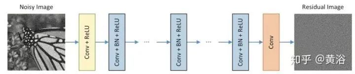
The figure shows the architecture of DnCNN. Given a depth of D, DnCNN has three types of layers. (i) Conv + ReLU: The first layer generates 64 feature maps with 64 filters of size 3×3×c, followed by ReLU, where c represents the number of channels in the image, c = 1 for grayscale images and c = 3 for color images. (ii) Conv + BN + ReLU: Layers 2 to (D-1) have 64 filters of size 3×3×64, with BN added between convolution and ReLU. (iii) Conv: The last layer has c filters of size 3×3×64 to reconstruct the output.

DnCNN employs residual learning to train the residual mapping R(y) ≈ v, leading to x = y – R(y). The DnCNN model has two main features: it uses residual learning to learn R(y) and incorporates BN to accelerate training and improve denoising performance. By combining convolution with ReLU, DnCNN gradually separates the image structure from noise interference through hidden layers. This mechanism is similar to the iterative noise elimination strategies used in methods like EPLL and WNNM, but DnCNN is trained in an end-to-end manner.

The network in the figure can be used to train the original mapping F(y) to predict x or the residual mapping R(y) to predict v. When the original mapping is more like the individual mapping, the residual mapping will be easier to optimize. Note that the noisy observation y resembles the potential clean image x rather than the residual image v (especially at low noise levels). Therefore, F(y) will be closer to the individual mapping than R(y), and the residual learning formula is more suitable for image denoising.

• CBD-Net

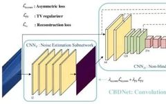
To enhance the robustness and practicality of deep denoising models, the Convolutional Blind Denoising Network (CBD-Net) combines several features, including network structure, noise modeling, and asymmetric learning. CBD-Net consists of a noise estimation subnet and a denoising subnet, trained using a more realistic noise model that considers signal-dependent noise and camera internal processing pipelines. Non-blind denoisers (e.g., the well-known BM3D) can be sensitive to errors in noise estimation, allowing the noise estimation subnet to suppress underestimated noise levels. To make the learned model applicable to real images, CBDNet is trained on synthetic images based on realistic noise models combined with nearly noise-free real images.

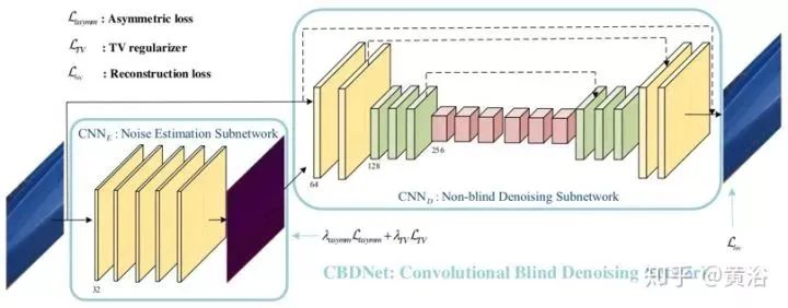
The figure shows the architecture of CBDNet for blind denoising. The noise model plays a crucial role in the CNN-based denoising performance. Given a clean image x, a more realistic noise model n(x) ~ N(0, σ(y)) can be expressed as follows:

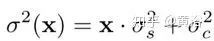
Here, n(x) = ns(x) + nc consists of the signal-dependent noise component ns and the stationary noise component nc. The nc is modeled as AWGN with noise variance σc², but for each pixel i, the noise variance of ns is correlated with the image intensity, i.e., x(i)·σs².

CBDNet includes a noise estimation subnet CNNE and a non-blind denoising subnet CNND. First, the noise estimation subnet CNNE takes the noisy observation y to produce an estimated noise level map σˆ(y) = FE(y; WE), where WE represents the network parameters of CNNE. The output of CNNE is a noise level map, as it has the same size as the input y, and is generated through a fully convolutional network. Then, the non-blind denoising subnet CNND takes both y and σˆ(y) as inputs to obtain the final denoised result x = FD(y, σ(y); WD), where WD represents the network parameters of CNND. Additionally, CNNE allows the estimated noise level map σ(y) to be adjusted before being fed into the non-blind denoising subnet CNND. A simple strategy is to let ρˆ(y) = γσˆ(y) to perform denoising calculations interactively.

The noise estimation subnet CNNE is a five-layer fully convolutional network without pooling and batch normalization (BN) operations. Each convolution layer has 32 feature channels and a filter size of 3×3. Each convolution layer is followed by ReLU. In contrast to CNNE, the non-blind denoising subnet CNND adopts a U-Net architecture, taking y and σˆ(y) as inputs to predict the noise-free clean image x. Residual learning is used to learn the residual mapping R(y, σˆ(y); WD) and then predict x = y + R(y, σˆ(y); WD). The 16-layer U-Net architecture of CNNE introduces symmetric skip connections, strided convolutions, and transposed convolutions to leverage multi-scale information and expand the receptive field. All filter sizes are 3×3, except for the last one, with ReLU added after each convolution layer.

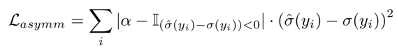
The following asymmetrical loss, defined as follows, is introduced into the noise estimation subnet and combined with the reconstruction loss to train the complete CBDNet:

Moreover, a total variation (TV) regularization is introduced to constrain the smoothness of σˆ(y),

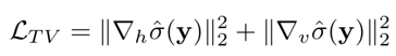
where ∇h (∇v) denotes the gradient operator in the horizontal (vertical) direction.

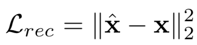
The reconstruction loss is

The total loss function is

Some example results:

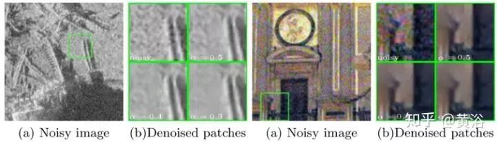
Image Dehazing

Single image dehazing is a challenging ill-posed problem. Existing methods use various constraints/priors to obtain seemingly reasonable dehazing solutions. The key to achieving dehazing is estimating the medium transmission map of the input hazy image.

• DehazeNet

DehazeNet is a trainable end-to-end system for medium transmission estimation. DehazeNet takes hazy images as input and outputs their medium transmission maps, subsequently recovering haze-free images through the atmospheric scattering model. DehazeNet employs a deep CNN architecture designed to embody the assumptions/priors of image dehazing. Specifically, Maxout units are used for feature extraction, capturing nearly all haze-related features. A new nonlinear activation function, called Bilateral Rectified Linear Unit (BReLU), improves the quality of haze-free recovery.

The figure below shows the architecture of DehazeNet. Conceptually, DehazeNet consists of four sequential operations (feature extraction, multi-scale mapping, local maxima, and nonlinear regression), comprising three convolutional layers, max pooling, Maxout units, and BReLU activation functions. The details of the four operations are introduced below.

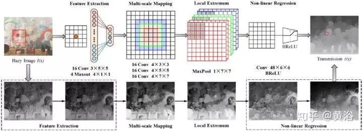
1) Feature extraction: To address the ill-posed nature of the image dehazing problem, various assumptions have been proposed, and based on these assumptions, haze-related features are densely extracted in the image domain, such as the well-known dark channel, color attenuation, and tone difference; thus, Maxout units with special activation functions are selected for dimensionality reduction and nonlinear mapping; Maxout is typically used as a simple feedforward nonlinear activation function in multi-layer perceptrons (MLP) or CNNs; when used in CNNs, pixel-wise maximization operations are performed on k affine feature maps to generate new feature maps; the design of the first layer of DehazeNet is as follows

where

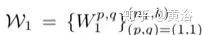
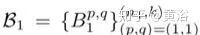
represent filters and biases, respectively.

2) Multi-scale mapping: Multi-scale features have been shown to be effective for haze removal; multi-scale feature extraction achieves scale invariance effectively; it is chosen to use parallel convolution operations in the second layer of DehazeNet, where any convolution filter size is between 3×3, 5×5, and 7×7, so the output of the second layer is written as

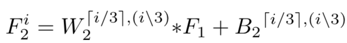
where

includes n2 groups of parameters, n2 is the output dimension of the second layer, i∈[1, n2] indexes the output feature maps, ⌈⌉ indicates the ceiling operation representing the remainder operation.

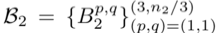
3) Local maxima: According to the classic architecture of CNNs, considering the maximum value in the neighborhood at each pixel can overcome local sensitivity; additionally, local maxima are based on the assumption of local constancy of the medium transmission and are typically used to overcome noise in transmission estimation; the third layer uses local maxima operations, namely

Note: Local maxima are densely applied to feature maps, which can maintain image resolution.

4) Nonlinear regression: Standard choices of nonlinear activation functions include Sigmoid and ReLU; the former is susceptible to gradient vanishing, leading to slow convergence of network training or local optima; hence, ReLU was proposed as a sparse representation method; however, ReLU only suppresses output when values are less than zero, which may lead to response overflow, especially in the last layer; thus, a BReLU activation function is adopted, as shown in the figure; BReLU maintains bilateral restraint and local linearity; thus, the fourth layer feature map is defined as

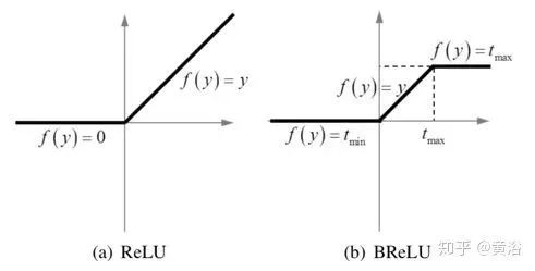
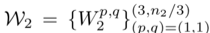
Here, W4 = {W4} contains filters of size n3×f4×f4, and B4 = {B4} contains biases, where tmin, max are the marginal values of BReLU (tmin = 0 and tmax = 1). According to the above formula, the gradient of this activation function can be expressed as

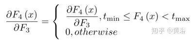
By cascading the aforementioned four layers, a trainable end-to-end system based on CNN is formed, where the filters and biases associated with convolutional layers are the network parameters to be learned.

• EPDN

The paper simplifies the image dehazing problem to an image-to-image translation problem and proposes the Enhanced Pix2pix Dehazing Network (EPDN), which can generate haze-free images without relying on physical scattering models. EPDN embeds a Generative Adversarial Network (GAN) followed by an enhancer. One theory posits that visual perception is globally prioritized, so the discriminator guides the generator to create pseudo-realistic images at a coarse scale, while the enhancer behind the generator needs to produce realistic dehazed images at a fine scale. The enhancer consists of two enhancement blocks based on the receptive field model, enhancing color and detail in the dehazing effect. Furthermore, the embedded GAN is trained together with the enhancer.

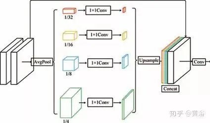
The figure shows a schematic diagram of the EPDN architecture, consisting of a multi-resolution generator module, an enhancer module, and a multi-scale discriminator module. Even though pix2pixHD uses coarse-to-fine features, the results still lack detail and exhibit color oversaturation. One possible reason is that existing discriminators are limited in guiding generators to create real details. In other words, the discriminator should only guide the generator to recover structures rather than details. To effectively address this issue, a pyramid pooling module is employed to ensure that feature details at different scales are embedded into the final result, i.e., the enhancement block. From the global contextual information of target recognition, it is evident that feature details are needed at various scales. Therefore, the enhancement block is designed based on the receptive field model to extract information at different scales.

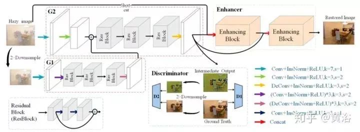
The figure shows the architecture of the enhancement block: there are two 3×3 front-end convolution layers, with the outputs of the front-end convolution layers reduced by factors of 4×, 8×, 16×, and 32×, thus constructing a four-scale pyramid; feature maps at different scales provide different receptive fields, aiding in image reconstruction at varying scales; then, a 1×1 convolution is used for dimensionality reduction, which effectively implements an adaptive weighted channel attention mechanism; subsequently, the feature maps are upsampled to the original size and connected with the outputs of the front-end convolution layers; finally, a 3×3 convolution is performed on the connected feature maps.

In EPDN, the enhancer consists of two enhancement blocks. The input of the first enhancement block is the connection of the original image and the features from the generator, while these feature maps are also input to the second enhancement block.

• PMS-Net

The Patch Map Selection Network (PMS-Net) is an adaptive and automated patch size selection model that primarily selects the patch size corresponding to each pixel. The network is designed based on CNN and can generate patch maps from the input image. Its dehazing algorithm flowchart is shown in the figure.

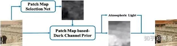
To enhance the performance of this network, PMS-Net proposes a pyramid-style multi-scale U-module. Based on the patch map, it can predict more accurate atmospheric light and transmission maps. The proposed architecture can avoid the problems of traditional DCP (e.g., incorrect recovery in bright or white scenes), restoring image quality superior to other algorithms. Among them, a patch map is defined to address the fixed patch size issue of the dark channel prior (DCP).

The figure shows the architecture of PMS-Net, divided into an encoder and a decoder. Initially, the input hazy image and 16 convolutional filters of size 3×3 are projected into a higher-dimensional space. Then, the multi-scale U-module extracts features from the higher-dimensional data. The design of the multi-scale U-module is shown in the left side of the figure.

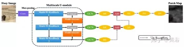
The input will pass through several Multiscale-W-ResBlocks (MSWR), as shown in the left side of the figure. The design idea of MSWR is similar to Wide-ResNet (WRN), improving ResNet by increasing the network width and reducing depth. Each block performs a series of operations, including Conv-BN-ReLU-Dropout-Conv-BN-ReLU, using shortcuts to extract information. The multi-scale concept in MSWR is similar to Inception-ResNet, employing multi-layer techniques to enhance the diversity of information and extract details.

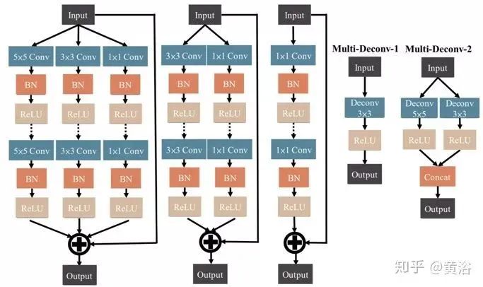
In the other parts of the multi-scale U-module, the Multi-Deconv module connects information with MSWR rather than the output of the transposed convolution, as the transposed convolution layers can help the network reconstruct the shape information of the input data. Therefore, through multi-scale transposed convolution combinations, more accurate feature maps can be reconstructed from the front layers of the network. Additionally, Multi-Deconv performs pyramid-style operations and enhances the scale to connect with MSWR. That is, feature maps from different layers run deconvolution at different scales (see the multi-scale U-module figure on the right).

To preserve high resolution, the outputs of the MSWR and Multi-Deconv modules are directly connected. Then, the feature maps are fed into the higher layers of the network’s Multi-Deconv module and decoder. The decoder adopts global convolutional network modules (GCN). A boundary refinement module (BR) is also used to retain edge information. Upsampling operations upgrade the scale layers. Additionally, a dense connection style is employed to merge high and low-resolution information. PMS-Net can predict patch maps.

The figure shows some analysis of experimental results: a comparison of dehazing results in white and bright scenes; Column 1: Input image; Column 2: Results from fixed-size patch DCP; Column 3: Results from the PMS-Net method; Column 4: Enlargements of white or bright areas in Columns 2 and 3; Column 5: Patch map; Columns 6-7: Medium transmission maps estimated by DCP and PMS-Net methods, respectively.

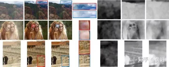
Image Deblurring

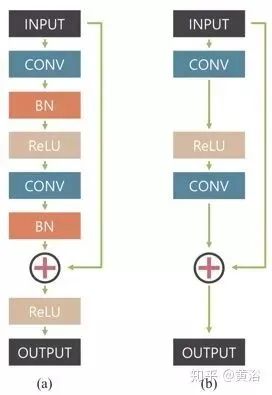
This is a multi-scale convolutional neural network that restores clear images in an end-to-end manner, where blurriness is caused by various sources, including lens motion, scene depth, and object motion. The figure shows the defined network model architecture, called ResBlocks: (a) the original residual network building block, (b) the modular building block modified by this network; batch normalization (BN) layers are not used because the mini-batch size for training the model is 2, which is smaller than what BN usually requires; removing the ReLU before the output is beneficial for improving empirical performance.

The designed deblurring multi-scale network architecture is shown in the figure below: Bk, Lk, Sk represent the blurry, potential, and GT clear images, respectively. The subscript k indicates the k-th scale layer of the Gaussian pyramid, downsampled to a scale of 1 / 2k. The model takes the blurry image pyramid as input and outputs the estimated potential image pyramid. Each intermediate scale’s output is trained to be clear. During testing, the output image at the original scale is selected as the final result.

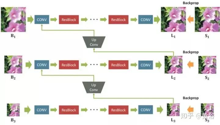
A sufficient number of convolutional layers are stacked with ResBlocks to expand the receptive field for each scale. During training, the resolution of the Gaussian pyramid patches for input and output is set to {256×256, 128×128, 64×64}. The scale ratio between consecutive scales is 0.5. The filter size for all convolution layers is 5×5. Since the model is fully convolutional, the patch sizes may vary during testing.

A multi-scale loss function is defined to simulate the traditional coarse-to-fine approach

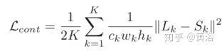
where Lk and Sk represent the model output image and GT image at scale layer k, respectively. The adversarial loss function is defined as

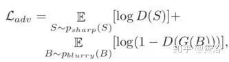
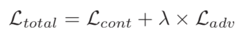
where G and D are the generator and discriminator, respectively. The final loss function is

Some results are shown in the figure, with several scaled local details.

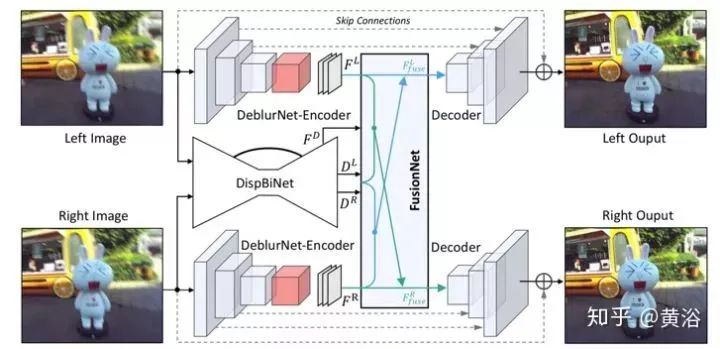
The Depth Awareness and View Aggregation Network (DAVANet) is a stereo image deblurring network. The network integrates depth and variation information from two views of a 3D scene, helping to eliminate complex spatial variation blurriness in dynamic scenes. Specifically, through this fusion network, bidirectional disparity estimation and deblurring are integrated into a unified framework.

The figure describes the blurriness caused by stereo vision: (a) is the depth variation blur caused by relative translation parallel to the image plane, (b) and (c) are perspective variation blurs caused by relative translation and rotation along the depth direction. Note that all complex motions can be decomposed into these three pairs of motion patterns.

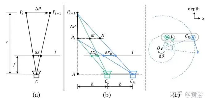
As shown in figure (a), we can obtain:

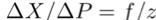
where ΔX, ΔP, f, and z represent the size of the blur, the motion of the target point, the focal length, and the depth of the target point, respectively.

As shown in figure (b), we know:

where b is the baseline, and h is the distance between the left camera CL and the line segment PtPt+1.

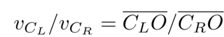
As shown in figure (c), the speeds of the two lenses vCL and vCR are proportional to the respective rotation radii CLO and CRO, i.e.,

The overall flowchart of DAVANet is shown in the figure, consisting of three sub-networks: DeblurNet for single-lens deblurring, DispBiNet for bidirectional disparity estimation, and FusionNet that adaptively selects and integrates depth and dual-view information. Here, small convolutional filters (3×3) are used to construct these three sub-networks, as large filters do not improve performance.

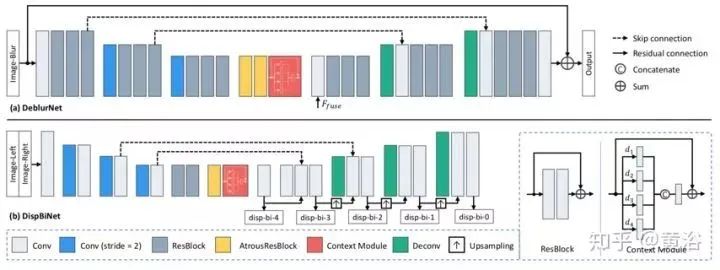
The structure of DeblurNet is based on U-Net, as shown in figure (a). Using basic residual modules as building blocks, the encoder outputs features reduced to 1/4×1/4 of the input size. Subsequently, the decoder reconstructs the clear image at full resolution through two upsampling residual blocks. Skip connections are used between corresponding feature maps in the encoder and decoder. Additionally, residual connections between the input and output are employed. This makes it easier for the network to estimate the residual between blurry-sharp image pairs while maintaining color consistency. Also, two atrous residual blocks and a Context module are used between the encoder and decoder to obtain richer features. DeblurNet shares weights between the two views.

Inspired by the previous DispNet model structure, a small DispBiNet is adopted, as shown in figure (b). Unlike DispNet, DispBiNet can predict bidirectional disparity from a forward process. The output is at full resolution, with three downsampling and upsampling operations in the network. Additionally, DispBiNet employs residual blocks, atrous residual blocks, and Context modules.

To embed multi-scale features, both DeblurNet and DispBiNet utilize a Context module, which contains parallel dilated convolutions with different dilation rates (dilated rate), as shown in the figure. The four dilation rates are set to 1, 2, 3, and 4. The Context module merges richer hierarchical contextual information, aiding in deblurring and disparity estimation.

To utilize depth and dual-view information for deblurring, a Fusion Network is introduced to enrich features with disparity and dual view. As shown in the figure, FusionNet takes the original stereo images IL, IR, the estimated left view disparity DL, features FD from the second to last layer of DispBiNet, and features FL, FR from the encoder of DeblurNet as inputs to generate the fused left view feature FLfuse.

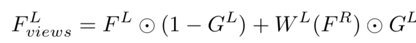
For dual view aggregation, the estimated left eye disparity DL deforms the right eye features FR of DeblurNet to the left eye, i.e., WL(FR). Instead of directly connecting WL(FR) and FL, a subnet GateNet generates a soft gate map (soft gate map) GL ranging from 0 to 1. The gate map can be adaptively selected to fuse features FL and WL(FR), i.e., selecting useful features while rejecting incorrect features from another view. For instance, in occlusion or erroneous disparity areas, the gate map value tends to be 0, indicating that only features from the reference view FL are used. GateNet consists of five convolution layers, as shown in the figure, where the input is the absolute difference between the left image IL and the deformed right image WL(IR), i.e., | IL – WL(IR)|, and the output is a single-channel gate map. All feature channels share the same gate map to generate aggregated features:

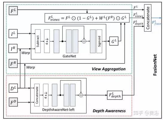
For depth awareness, a subnet DepthAwareNet with three convolution layers is used, and the two views do not share this subnet. Given the disparity DL and features FD from the second to last layer of DispBiNet, DepthAwareNet-left generates depth-associated features FL. In fact, DepthAwareNet implicitly learns prior knowledge of depth awareness, which helps in deblurring dynamic scenes.

Finally, the original left image features FL, view aggregation features FLviews, and depth-aware features FLdepth are connected to generate the fused left view feature FLfuse. Similarly, the same architecture as FusionNet can be used to obtain the fused features for the right view.

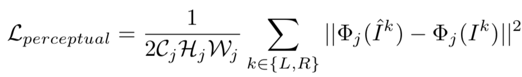
The loss function for DeblurNet includes two parts: MSE loss and perceptual loss, namely

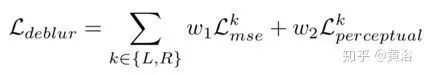
where

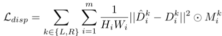
The disparity loss function for DispBiNet is as follows:

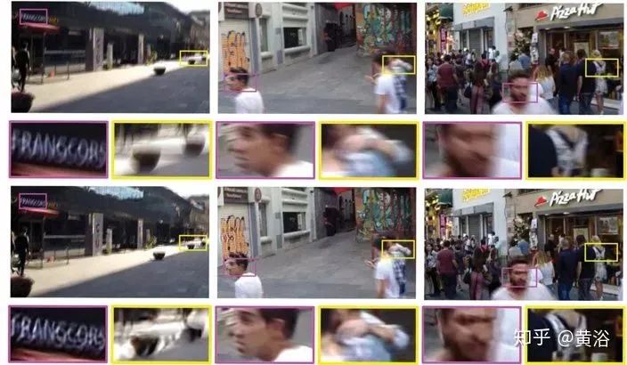
The figure shows the role of disparity in deblurring: (a), (f), (g), and (h) respectively represent the blurry image, the clear image, the predicted disparity, and the GT disparity. (b) and (e) are the results from the monocular deblurring network DeblurNet and the binocular deblurring network DAVANet, respectively. In (c), two left images are input, and DispBiNet cannot provide any depth information or disparity for depth awareness and view aggregation. In (d), to eliminate the influence of view aggregation, features from other views are not deformed from FusionNet. Since this network can accurately estimate and utilize disparity, its performance surpasses other methods.

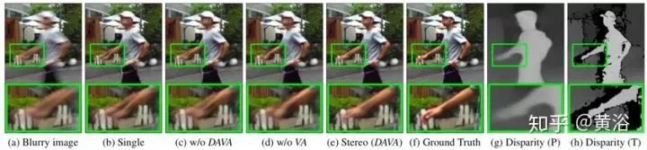
Image Enhancement

• Deep Bilateral Learning

This is a neural network architecture for image enhancement, inspired by bilateral grid processing and local affine color transformations. Based on input/output image pairs, the convolutional neural network is trained to predict the coefficients of the local affine model in bilateral space. The goal of the network architecture is to learn how to make local, global, and content-dependent decisions to approximate the desired image transformation. The input to the neural network is a low-resolution image, generating a set of affine transformations in bilateral space, which are then upsampled in an edge-preserving manner and transformed into a full-resolution image. The model is trained offline from data and does not require access to the original operations at runtime. This allows the model to learn complex, scene-dependent transformations.

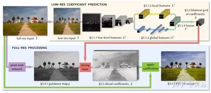
As shown in the figure, the low-resolution input I executes most of the inference (top of the figure), similar to bilateral grid methods, ultimately predicting local affine transformations. Image enhancement typically depends not only on local image features but also on global image features, such as histograms, average intensity, and even scene categories. Therefore, the low-resolution stream is further divided into local and global paths. Merging these two paths generates coefficients representing the affine transformation.

The high-resolution stream (bottom of the figure) operates in full-resolution mode, performing minimal computation but effectively capturing high-frequency effects and preserving edges. To this end, a slicing node is introduced. This node performs data-dependent lookups at the low-resolution grid points for the constrained coefficients based on the learned guidance map. Based on the full-resolution guidance map, high-resolution affine coefficients obtained from the grid slices are used to perform local color transformations for each pixel, producing the final output O. During training, the loss function is minimized at full resolution. This means that while processing a large amount of downsampled data in the low-resolution stream, the model can still learn intermediate features and affine coefficients that reproduce high-frequency effects.

Below are some examples showing the effects of various improvements. As shown in the figure, the low-level convolution layers have learning capabilities to extract semantic information. Replacing these layers with standard bilateral grid splatting operations would result in a significant loss of network expressiveness.

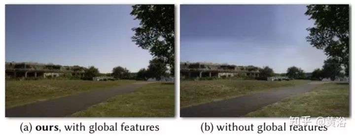
As shown in the figure, the global feature path allows the model to infer the complete image, (a) for example, reproducing adjustments based on intensity distribution or scene type. (b) Without the global path, the model may make spatially inconsistent local decisions.

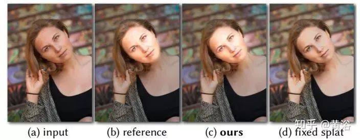
As shown in the figure, the new slicing node is crucial for the expressiveness of the architecture and its handling of high-resolution effects. Replacing this node with transposed convolution filters would reduce expressiveness (b), as no full-resolution data is used to predict output pixels. Due to the full-resolution guidance map, the slicing layer approximates with higher fidelity (c).

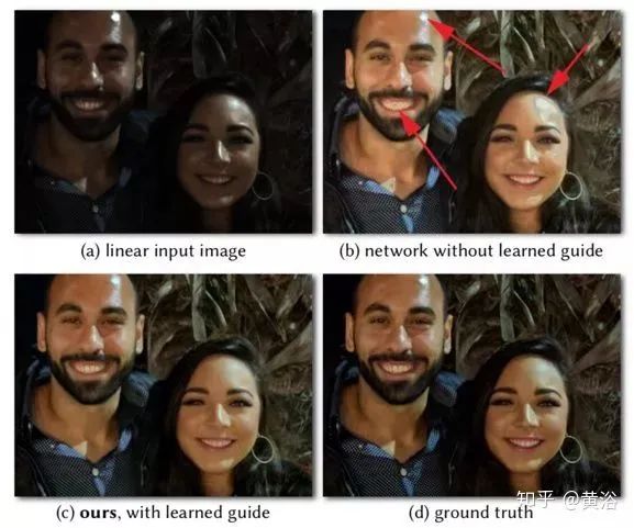
As shown in the figure, (b) HDR brightness distortion, especially posterization artifacts in the highlights on the forehead and cheeks. In contrast, the guidance map of the slicing node allows (c) to reproduce (d) the underlying ground truth GT correctly.

• Deep Photo Enhancer

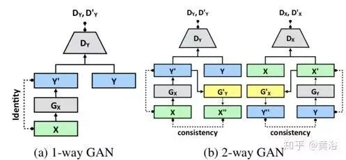
It proposes an unpaired learning approach for image enhancement. Given a set of photos with desired features, this method learns a photo enhancer that transforms input images into enhanced images with these features. Based on a two-way Generative Adversarial Network (GAN) framework, improvements are as follows: 1) The global feature-augmented U-Net is used, where the global U-Net serves as the generator of the GAN model; 2) An adaptive weighting scheme improves Wasserstein GAN (WGAN), leading to faster convergence and better training stability with lower sensitivity to parameters than WGAN-GP; 3) The generator of the two-way GAN employs separate BN layers, aiding the generator in better adapting to its input distribution and enhancing the stability of GAN training.

The figure introduces the architecture of the two-way GAN. (a) is the architecture of a one-way GAN. Given input x∈X, the generator GX transforms x into y’ = GX(x)∈Y. The discriminator DY aims to distinguish samples in the target domain {y} from generated samples {y’ = GX(x)}. To achieve cycle consistency, a two-way GAN is adopted, such as CycleGAN and DualGAN. They require G’Y(GX(x)) = x, where the generator G’Y takes the samples generated by GX and maps them back to the source domain X. Additionally, the two-way GAN typically includes forward mapping (X → Y) and backward mapping (Y → X). (b) shows the architecture of the two-way GAN. During forward propagation,

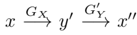
to check consistency between x” and x. During backward propagation,

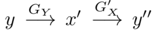
to check consistency between y and y”.

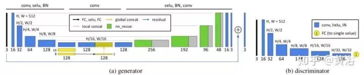
The figure shows the architecture of the generator and discriminator of the GAN. The generator is based on U-Net but adds global features. To improve model efficiency, the extraction of global features shares the first five layers of local feature extraction with the contracting part of U-Net. Each contraction step includes 5×5 filtering, a stride of 2, SELU activation, and BN. For global features, it is assumed that the fifth layer is a 32×32×128 feature map, further reduced to 16×16×128 and then 8×8×128 after contracting. Through a fully connected layer, a SELU activation layer, and another fully connected layer, the 8×8×128 feature map is reduced to 1×1×128. The extracted 1×1×128 global features are then replicated into 32×32 copies and concatenated with the low-level features of size 32×32×128 to obtain a 32×32×256 feature map, which simultaneously merges local and global features. The U-Net expansion path is executed on the merged feature map. Finally, the idea of residual learning is adopted, meaning the generator only learns the differences between the input image and the labeled image.

WGAN relies on the Lipschitz constraint of the training objective: a differentiable function is 1-Lipschitz if and only if its gradient norm is at most 1. To meet the constraint, WGAN-GP directly constrains the output gradient of the discriminator with respect to its input by adding the following gradient penalty,

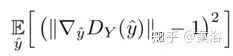
where yˆ is a sampled point along the line between the target distribution and the generator distribution.

The parameter λ weights the penalty added to the original discriminator loss. λ determines the trend of the gradient approaching 1. If λ is too small, the Lipschitz constraint cannot be guaranteed. On the other hand, if λ is too large, convergence may be slow because the penalty may overweight the discriminator loss. The choice of λ is crucial. Conversely, using the following gradient penalty,

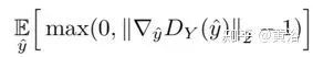
This better reflects the requirement that the gradient be less than or equal to 1 and only penalizes the part greater than 1 for the Lipschitz constraint. More importantly, an adaptive weighting scheme can be used to adjust the weight λ, selecting appropriate weights such that the gradients are within the desired range, such as [1.001, 1.05]. If the moving average of gradients within a sliding window (size = 50) exceeds the upper limit, it indicates that the current weight λ is too small and the penalty force is insufficient to ensure the Lipschitz constraint. Therefore, λ can be doubled to increase the weight. On the other hand, if the moving average of gradients is below the lower limit, then λ can be halved to prevent it from becoming too large. This improvement is called A-GAN (Adaptive GAN).

The previous figure (a) serves as GX for the generator, while figure (b) serves as DY for the discriminator, obtaining the architecture of the one-way GAN in the previous figure (a). Similarly, generalizing A-GAN can yield the two-way GAN architecture as shown in the previous figure (b).

• Deep Illumination Estimation

This is a method based on neural networks to enhance underexposed photos, introducing intermediate illumination that associates input with expected enhanced results, thereby strengthening the network’s ability to learn complex photographic retouching processes from expert-modified input/output image pairs. Based on this model, a loss function is defined with illumination constraints and priors, training the network to effectively learn the retouching processes under various lighting conditions. Through these methods, the network can recover clear details, vivid contrasts, and natural colors.

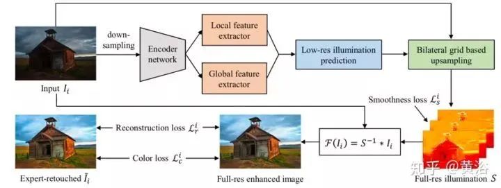
Fundamentally, the image enhancement task can be referred to as finding a mapping function F, enhancing the input image I such that Ĩ = F(I) is the desired image. In the Retinex image enhancement method, the inverse of F is typically modeled as an illumination map S, which pixel-wise multiplies with the reflectance image Ĩ to produce the observed image I: I = S * Ĩ.

The reflectance component Ĩ can be viewed as an exposure-appropriate image; thus, in the model, Ĩ serves as the enhanced result, while I serves as the observed underexposed image. Once S is known, the enhanced result Ĩ can be obtained via F(I) = S⁻¹ * I. S is modeled as multi-channel (R, G, B) data rather than single-channel data to enhance its capability in color enhancement, especially in handling the nonlinear characteristics of different color channels.

The figure is a pipeline diagram of the network. Enhancing underexposed photos requires adjusting local (contrast, detail clarity, shadows, and highlights) and global features (color distribution, average brightness, and scene categories). Considering the local and global contextual information generated by the encoder network, see the upper part of the figure. To drive the network to learn the illumination mapping from the input underexposed image (Ii) to the corresponding expert-modified image (Ĩ), a loss function is designed, incorporating illumination smoothness priors and enhanced reconstruction and color losses, as shown in the lower part of the figure. These strategies effectively learn S from (Ii, Ĩi) through a variety of photo adjustments to recover the enhanced image. Notably, this method learns local and global features of the predicted image-illumination mapping at low resolution while upsampling the low-resolution predictions to full resolution based on bilateral grids, ensuring good system real-time performance.

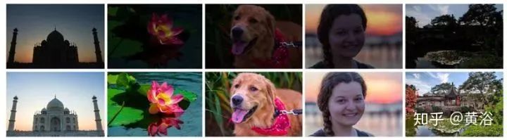
Below are some examples of enhanced results (top: input, bottom: enhanced).

References

• 1. K Zhang et al., “Beyond a Gaussian denoiser: Residual learning of deep CNN for image denoising”, IEEE T-IP, 2017

• 2. A Ignatov et al., “DSLR-Quality Photos on Mobile Devices with Deep Convolutional Networks“, arXiv 1704.02470, 2017

• 3. P. Svoboda et al., “Compression artifacts removal using convolutional neural networks”. arXiv 1605.00366, 2016.

• 4. B. Cai et al.,”Dehazenet: An end-to-end system for single image haze removal”. IEEE T-IP, 2016

• 5. X. Mao, C. Shen, Y.-B. Yang. “Image restoration using very deep convolutional encoder-decoder networks with symmetric skip connections”. Advances in Neural Information Processing Systems 29, 2016

• 6. Z. Yan et al., “Automatic photo adjustment using deep neural networks”. ACM Trans. Graph., 2016

• 7. M Gharbi et al.,“Deep Bilateral Learning for Real-Time Image Enhancement”, arXiv 1707.02880, 2017

• 8. S Nah, T Kim, K Lee,“Deep Multi-scale Convolutional Neural Network for Dynamic Scene Deblurring”, CVPR, 2017

• 9. Y Chen et al.,“Deep Photo Enhancer: Unpaired Learning for Image Enhancement from Photographs with GANs”, CVPR, 2018.

• 10. J Zhang et al., “Dynamic Scene Deblurring Using Spatially Variant Recurrent Neural Networks”, CVPR 2018.

• 11. S Guo et al.,“Toward Convolutional Blind Denoising of Real Photographs”, CVPR, 2019

• 12. R Wang et al.,“Underexposed Photo Enhancement using Deep Illumination Estimation”, CVPR 2019.

• 13. Y Qu et al.,“Enhanced Pix2pix Dehazing Network”, CVPR, 2019

• 14. S Zhou et al.,“DAVANet: Stereo Deblurring with View Aggregation”, CVPR 2019.

• 15. W Chen, J Ding, S Kuo,“PMS-Net: Robust Haze Removal Based on Patch Map for Single Images”, CVPR, 2019

Download 1: OpenCV-Contrib Chinese Tutorial

Reply "OpenCV Contrib Chinese Tutorial" in the background of the "Beginner Learning Vision" public account to download the first OpenCV Contrib tutorial in Chinese on the internet, covering more than twenty chapters including installation of extension modules, SFM algorithms, stereo vision, target tracking, biological vision, and super-resolution processing.

Download 2: Python Vision Practical Projects 52 Lectures

Reply "Python Vision Practical Projects" in the background of the "Beginner Learning Vision" public account to download 31 vision practical projects including image segmentation, mask detection, lane line detection, vehicle counting, eyeliner addition, license plate recognition, character recognition, emotion detection, text content extraction, and face recognition, to help quickly learn computer vision.

Download 3: OpenCV Practical Projects 20 Lectures

Reply "OpenCV Practical Projects 20 Lectures" in the background of the "Beginner Learning Vision" public account to download 20 practical projects based on OpenCV to advance OpenCV learning.

Discussion Group

Welcome to join the public account reader group to communicate with peers. Currently, there are WeChat groups for SLAM, 3D vision, sensors, autonomous driving, computational photography, detection, segmentation, recognition, medical imaging, GAN, algorithm competitions, etc. (which will be gradually subdivided in the future). Please scan the WeChat number below to join the group, and note: "Nickname + School/Company + Research Direction", for example: "Zhang San + Shanghai Jiao Tong University + Visual SLAM". Please follow the format for the note; otherwise, you will not be approved. Once successfully added, you will be invited to the relevant WeChat group based on your research direction. Please do not send advertisements in the group; otherwise, you will be removed from the group. Thank you for your understanding~