Artificial intelligence, like immortality and interstellar travel, is one of humanity’s greatest dreams. Although computer technology has made significant progress, no computer has yet been able to produce a “self” awareness. However, since 2006, the field of machine learning has made groundbreaking advancements. The Turing test is at least not as unreachable as it once seemed. As for the technical means, it relies not only on the parallel processing capabilities of cloud computing for big data but also on algorithms. This algorithm is called Deep Learning. With the help of the Deep Learning algorithm, humanity has finally found a way to tackle the ancient problem of processing “abstract concepts”.

Machine Learning is a discipline that studies how computers can simulate or achieve human learning behaviors to acquire new knowledge or skills, reorganizing existing knowledge structures to continuously improve their performance. In simple terms, Machine Learning uses algorithms to enable machines to learn patterns from a large amount of historical data, thereby intelligently recognizing new samples or predicting the future.
There are still many unresolved issues in the development of Machine Learning in areas such as image recognition, speech recognition, natural language understanding, weather forecasting, gene expression, and content recommendation.
Traditional pattern recognition methods involve obtaining data through sensors, followed by preprocessing, feature extraction, feature selection, and then reasoning, prediction, or recognition.
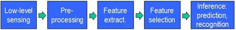
Initially, data is obtained through sensors (e.g., CMOS). Then it goes through preprocessing, feature extraction, feature selection, and finally reasoning, prediction, or recognition. The last part, which is the machine learning part, has most of the work done in this area, and there are many papers and studies available.
The three middle parts can be summarized as feature representation. Good feature representation plays a critical role in the accuracy of the final algorithm, and most of the system’s computational and testing work is consumed in this large part. However, this part is generally completed manually, relying on human feature extraction. Manual feature selection is time-consuming and labor-intensive, requiring expertise and largely relying on experience and luck. So, can machines learn features automatically? The emergence of Deep Learning provides a solution to this problem.
The visual mechanism of the human brain
The 1981 Nobel Prize in Physiology or Medicine was awarded to David Hubel (a Canadian-born American neurobiologist) and Torsten Wiesel, as well as Roger Sperry. The main contribution of the first two was the “discovery of the information processing of the visual system,” indicating that the visual cortex is hierarchical.
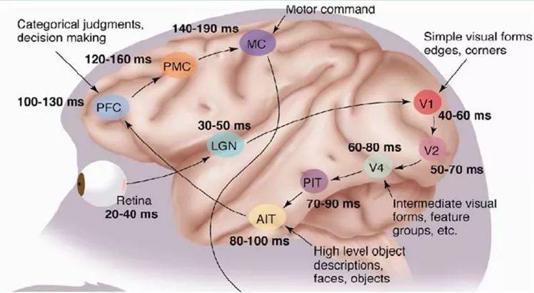
In 1958, David Hubel and Torsten Wiesel at Johns Hopkins University studied the correspondence between the pupil region and the neurons in the cerebral cortex. They made a 3mm hole in the skull of a cat and inserted electrodes to measure the activity level of the neurons.
Then, they presented various shapes and brightness levels of objects in front of the kitten. Additionally, they changed the position and angle of each object presented. They hoped that this method would allow the kitten’s pupils to perceive different types and intensities of stimuli.
The purpose of this experiment was to prove a hypothesis. There exists a correspondence between different visual neurons in the posterior cortex and the stimuli received by the pupil. Once the pupil is stimulated by a certain type of stimulus, a specific part of the neurons in the posterior cortex becomes active. After many days of tedious experiments, David Hubel and Torsten Wiesel discovered a type of neuron cell called “Orientation Selective Cell.” This type of neuron becomes active when the pupil detects the edge of an object in front of it, and this edge points in a certain direction.
This discovery sparked further thoughts about the nervous system. The process of the nerve-central-brain may be a continuously iterative and abstract process.
For example, starting from the input of raw signal (pupil receiving pixel data), followed by preliminary processing (some cells in the cerebral cortex detect edges and directions), then abstraction (the brain determines that the shape of the object in front is circular), and further abstraction (the brain further determines that the object is a balloon).
This physiological discovery led to the groundbreaking development of artificial intelligence in the following forty years.
In general, the information processing of the human visual system is hierarchical. From low-level V1 region extracting edge features, to V2 region recognizing shapes or parts of targets, and then to higher levels, the entire target and its behaviors. This means that high-level features are combinations of low-level features, and the representation of features from low to high becomes increasingly abstract, capable of expressing semantics or intentions. The higher the level of abstraction, the fewer possible guesses exist, which facilitates classification. For example, the correspondence between a collection of words and sentences is many-to-one, and the correspondence between sentences and semantics is also many-to-one, as is the correspondence between semantics and intentions; this is a hierarchical system.
Features of Machine Learning
Features are the raw materials of a machine learning system, and their impact on the final model is indisputable. If the data is well represented as features, linear models can often achieve satisfactory accuracy.
Granularity of Feature Representation
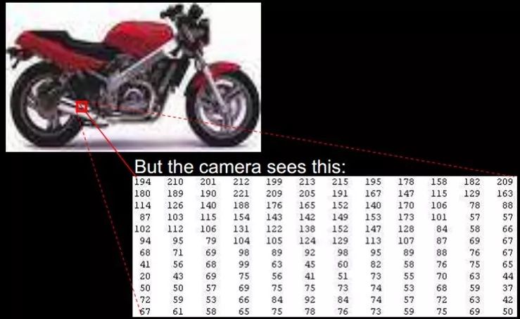
At what granularity can the learning algorithm’s feature representation function? For an image, pixel-level features are of no value. For instance, consider the motorcycle below; at the pixel level, no information can be obtained, and it cannot distinguish between motorcycles and non-motorcycles. However, if the features are structural (or meaningful), such as whether it has a handlebar, or whether it has wheels, it becomes easy to distinguish between motorcycles and non-motorcycles, allowing the learning algorithm to function.
Shallow Feature Representation
Since pixel-level feature representation is ineffective, what kind of representation is useful?
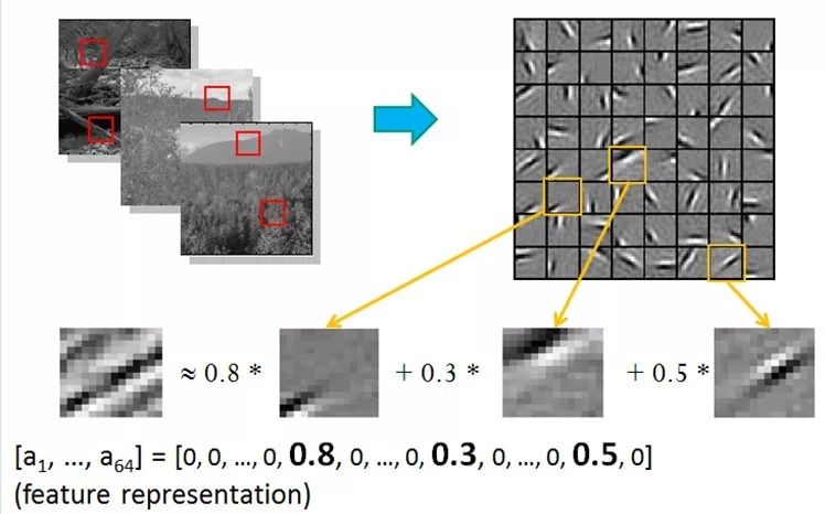
Around 1995, scholars Bruno Olshausen and David Field at Cornell University attempted to study visual problems using both physiological and computational methods.
They collected many black and white landscape photos and extracted 400 small fragments, each measuring 16×16 pixels, which we can label as S[i], i = 0,.. 399. Next, they randomly extracted another fragment from these black and white landscape photos, also measuring 16×16 pixels, which we can label as T.
The question they posed was how to select a group of fragments from these 400, S[k], to synthesize a new fragment that should be as similar as possible to the randomly selected target fragment T, while using as few S[k] as possible. In mathematical terms, this can be described as: Sum_k (a[k] * S[k]) –> T, where a[k] is the weight coefficient when synthesizing fragment S[k].
To solve this problem, Bruno Olshausen and David Field invented an algorithm known as Sparse Coding.
Sparse coding is a repeated iterative process, where each iteration consists of two steps:
1) Select a group of S[k] and then adjust a[k] to make Sum_k (a[k] * S[k]) as close to T as possible.
2) Fix a[k] and select other more suitable fragments S’[k] from the 400 fragments to replace the original S[k], making Sum_k (a[k] * S’[k]) as close to T as possible.
After several iterations, the optimal combination of S[k] is selected. Interestingly, the selected S[k] are mostly edge lines of different objects in the photos, with similar shapes but differing in direction.
The results of Bruno Olshausen and David Field’s algorithm coincided with the physiological findings of David Hubel and Torsten Wiesel!
This means that complex shapes are often composed of some basic structures. For instance, the image below can be linearly represented using 64 orthogonal edges (which can be understood as orthogonal basic structures). For example, the sample x can be synthesized using three of the 64 edges with weights of 0.8, 0.3, and 0.5, while the other basic edges contribute nothing and are thus zero.
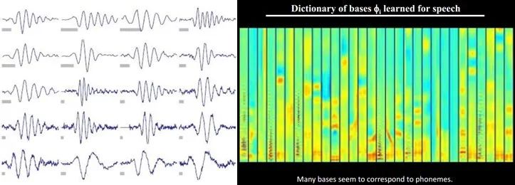
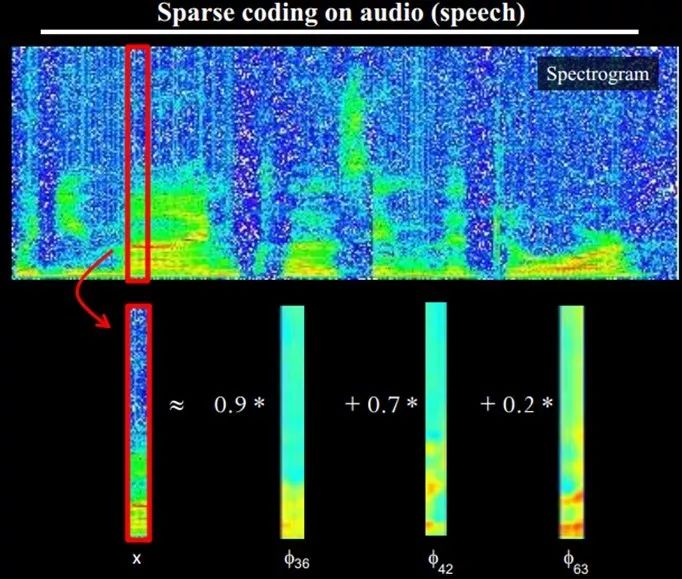
Moreover, this pattern exists not only in images but also in sounds. People have discovered 20 basic sound structures from unmarked sounds, and the rest of the sounds can be synthesized from these 20 basic structures.
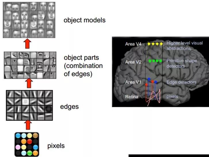
Structural Feature Representation
Small graphic blocks can be composed of basic edges, but how to represent more structured and complex, conceptual graphics? This requires higher-level feature representation, such as V2 and V4. Thus, V1 looks at the pixel level. V2 looks at V1 as pixel level, which is a hierarchical progression where high-level expressions are formed by the combination of low-level expressions. To be more technical, these are called bases. The base extracted from V1 is edges, then the V2 layer is a combination of these bases from the V1 layer, resulting in a higher-level base. The basis of the previous layer is again a combination of the bases from the layer before that… (This is why some experts say Deep Learning is about “getting bases”; because it sounds unpleasant, it is euphemistically called Deep Learning or Unsupervised Feature Learning).
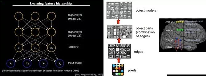
Intuitively speaking, it is about finding meaningful small patches and then combining them to obtain the features of the previous layer, recursively learning features upwards.
When training on different objects, the edge bases obtained are very similar, but the object parts and models can be completely different (which makes it much easier for us to distinguish between cars or faces).
We know that hierarchical feature construction is needed, from shallow to deep, but how many features should each layer have?
In any method, the more features there are, the more reference information is provided, which will improve accuracy. However, having too many features means increased computational complexity and larger exploratory space, leading to sparsity in the training data for each feature, which can bring various issues; thus, having more features does not necessarily mean better performance.
The Basic Idea of Deep Learning
Suppose we have a system S with n layers (S1,…Sn), where its input is I, and output is O, visually represented as: I =>S1=>S2=>…..=>Sn => O. If the output O equals the input I, meaning that no information is lost after the input I passes through this system (Haha, experts say this is impossible. There is a saying in information theory called “information loss layer by layer” (information processing inequality). If processing a results in b, and then processing b results in c, it can be proven that the mutual information between a and c will not exceed the mutual information between a and b. This indicates that information processing does not increase information; most processing will lose information. Of course, if the lost information is useless, that would be great), it means that the input I remains unchanged through each layer Si, representing the original information (i.e., input I) in another form. Now back to our topic of Deep Learning, we need to automatically learn features. Suppose we have a batch of inputs I (such as a batch of images or text), and we design a system S (with n layers), adjusting the parameters in the system so that its output remains the same as the input I. Then we can automatically obtain a series of hierarchical features of the input I, namely S1, …, Sn.
The idea of Deep Learning is to stack multiple layers, meaning that the output of one layer serves as the input of the next layer. In this way, hierarchical expression of input information can be achieved.
Additionally, the previous assumption that the output strictly equals the input is too strict; we can relax this condition slightly, for example, requiring only that the difference between input and output is as small as possible. This relaxation leads to another class of Deep Learning methods. The above describes the basic idea of Deep Learning.
Shallow Learning and Deep Learning
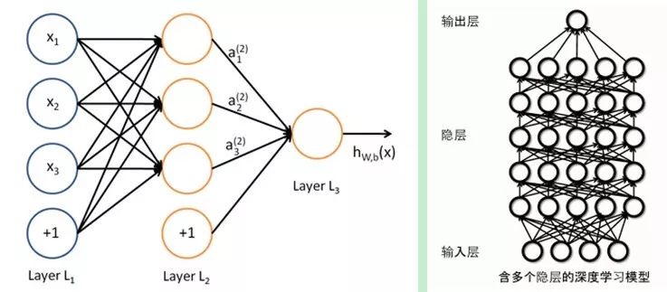
In the late 1980s, the invention of the backpropagation algorithm for artificial neural networks (also called the Back Propagation algorithm or BP algorithm) brought hope to machine learning, sparking a wave of machine learning based on statistical models that continues to this day. People discovered that using the BP algorithm allows an artificial neural network model to learn statistical patterns from a large number of training samples, thus predicting unknown events. This statistically-based machine learning method has shown advantages over previous systems based on manual rules in many aspects. At this time, artificial neural networks, although also referred to as multi-layer perceptrons (MLP), were essentially shallow models containing only one hidden layer of nodes.
In the 1990s, various shallow machine learning models were proposed, such as Support Vector Machines (SVM), Boosting, and Maximum Entropy methods (like Logistic Regression). The structures of these models can essentially be seen as having one hidden layer of nodes (like SVM, Boosting), or no hidden layers (like Logistic Regression). These models have achieved great success in both theoretical analysis and practical applications. In contrast, due to the difficulty of theoretical analysis and the need for much experience and skill in training methods, shallow artificial neural networks were relatively quiet during this period.
In 2006, Geoffrey Hinton, a professor at the University of Toronto and a leader in the field of machine learning, along with his student Ruslan Salakhutdinov, published an article in Science, initiating a wave of Deep Learning in academia and industry. This article had two main points: 1) Multi-hidden layer artificial neural networks have excellent feature learning capabilities, and the features learned provide a more essential characterization of the data, facilitating visualization or classification; 2) The difficulty of training deep neural networks can be effectively overcome through “layer-wise pre-training,” which is achieved through unsupervised learning.
Currently, most classification and regression learning methods are shallow structure algorithms, whose limitations lie in their ability to represent complex functions under limited samples and computational units, restricting their generalization capabilities for complex classification problems. Deep Learning can approximate complex functions by learning a deep nonlinear network structure, representing the distributed representation of input data, and demonstrating a strong ability to learn the essential features of data sets from a small number of samples (the benefit of having multiple layers is that complex functions can be represented with fewer parameters).
The essence of Deep Learning is to construct machine learning models with many hidden layers and massive training data to learn more useful features, ultimately improving the accuracy of classification or prediction. Therefore, “deep models” are a means, while “feature learning” is the goal. Unlike traditional shallow learning, the difference in Deep Learning lies in: 1) Emphasizing the depth of the model structure, typically having 5, 6, or even more than 10 hidden layers; 2) Highlighting the importance of feature learning, meaning that through layer-wise feature transformation, the features of samples in the original space are transformed into a new feature space, making classification or prediction easier. Compared to the manual rule-based feature construction methods, using big data to learn features can better characterize the rich intrinsic information of the data.
Deep Learning and Neural Networks
Deep Learning is a new field of research in machine learning, motivated by establishing and simulating the neural networks of the human brain for analytical learning. It mimics the mechanisms of the human brain to interpret data such as images, sounds, and text. Deep Learning is a form of unsupervised learning.
The concept of Deep Learning originates from the study of artificial neural networks. Multi-layer perceptrons with multiple hidden layers are a type of Deep Learning structure. Deep Learning combines low-level features to form more abstract higher-level representations, discovering the distributed feature representations of data.
Deep Learning itself is a branch of Machine Learning, which can be simply understood as the development of neural networks. About 20 to 30 years ago, neural networks were a particularly hot direction in the field of Machine Learning, but gradually faded away due to several reasons:
1) They are relatively easy to overfit, parameters are difficult to tune, and many tricks are needed;
2) Training speed is relatively slow, and under fewer layers (less than or equal to 3), their performance is not superior to other methods;
Thus, for about 20 years, neural networks received little attention, and during this time, SVMs and boosting algorithms dominated. However, a passionate old gentleman, Hinton, persisted and ultimately (along with others like Bengio and Yann LeCun) proposed a practically viable Deep Learning framework.
Deep Learning and traditional neural networks share similarities and differences:
The similarities lie in that Deep Learning adopts a hierarchical structure similar to neural networks, comprising an input layer, hidden layers (multiple), and an output layer. Only adjacent layer nodes are connected, while there are no connections between nodes in the same layer or across layers. Each layer can be considered a logistic regression model; this hierarchical structure closely resembles the structure of the human brain.
To overcome the training issues of neural networks, Deep Learning employs a training mechanism that is quite different from traditional neural networks. Traditional neural networks use the backpropagation method, which simply means using an iterative algorithm to train the entire network, randomly setting initial values, calculating the current network’s output, and then adjusting the parameters of previous layers based on the difference between the current output and the labels until convergence (the entire process is a gradient descent method). In contrast, Deep Learning generally adopts a layer-wise training mechanism.
The Training Process of Deep Learning
Using bottom-up unsupervised learning (training from the bottom layer upwards layer by layer)
Using unlabelled data (labelled data can also be used) to train the parameters of each layer, this step can be regarded as an unsupervised training process, which is the most significant difference from traditional neural networks (this process can be seen as a feature learning process):
Specifically, first train the first layer with unlabelled data, learning the parameters of the first layer (this layer can be seen as obtaining a hidden layer of a three-layer neural network that minimizes the difference between output and input). Due to the model capacity constraints and sparsity constraints, the resulting model can learn the structure of the data itself, thus obtaining features with greater representational capacity than the input; after learning the n-1 layer, the output of n-1 layer is used as the input for the n layer, training the n layer, and thus obtaining the parameters of each layer.
Top-down supervised learning (training with labelled data, error propagation from top to bottom, fine-tuning the network)
Based on the parameters obtained from the first step, further fine-tune the parameters of the entire multi-layer model in a supervised training process; the first step is similar to the random initialization process of neural networks, but since the first step of Deep Learning is not random initialization but is based on learning the structure of the input data, this initial value is closer to the global optimum, thus achieving better results; hence, the effectiveness of Deep Learning is largely attributed to the feature learning process of the first step.
CNNs: Convolutional Neural Networks
Convolutional neural networks are a type of artificial neural network and have become a research hotspot in the fields of speech analysis and image recognition. Its weight-sharing network structure makes it more similar to biological neural networks, reducing the complexity of the network model and the number of weights. This advantage is more apparent when the input is multi-dimensional images, allowing images to be input directly into the network, avoiding the complex feature extraction and data reconstruction processes in traditional recognition algorithms. Convolutional networks are a multi-layer perceptron specially designed for recognizing two-dimensional shapes, and this network structure has a high degree of invariance to translation, scaling, skewing, or other forms of deformation.
CNNs are influenced by early time-delay neural networks (TDNNs). Time-delay neural networks reduce learning complexity by sharing weights in the temporal dimension, suitable for processing speech and time series signals.
CNNs are the first truly successful learning algorithm to train multi-layer network structures. It reduces the number of parameters that need to be learned by utilizing spatial relationships to improve the training performance of the general forward BP algorithm. CNNs, as a deep learning architecture, are designed to minimize data preprocessing requirements. In CNNs, a small portion of the image (local receptive field) serves as the input for the lowest layer of the hierarchical structure, and information is sequentially transmitted to different layers, with each layer using a digital filter to obtain the most significant features of the observed data. This method can capture significant features of observations that are invariant to translation, scaling, and rotation, as the local receptive field of images allows neurons or processing units to access the most basic features, such as oriented edges or corners.
The History of Convolutional Neural Networks
In 1962, Hubel and Wiesel proposed the concept of receptive fields through their studies of cat visual cortex cells. In 1984, Japanese scholar Fukushima proposed the Neural Cognitive Machine based on the concept of receptive fields, which can be seen as the first implementation of convolutional neural networks and the first application of the receptive field concept in the field of artificial neural networks. The Neural Cognitive Machine decomposes a visual pattern into many sub-patterns (features) and then processes them in a hierarchically connected feature plane, attempting to model the visual system so that it can recognize objects even when they are displaced or slightly deformed.
Typically, the Neural Cognitive Machine includes two types of neurons: S-units that undertake feature extraction and C-units that resist deformation. S-units involve two important parameters: receptive field and threshold parameters; the former determines the number of input connections, while the latter controls the degree of response to feature sub-patterns. Many scholars have been dedicated to improving the performance of the Neural Cognitive Machine: in traditional Neural Cognitive Machines, the visual blurring caused by C-units in each S-unit’s receptive field follows a normal distribution. If the blurring effect at the edge of the receptive field is greater than that at the center, the S-unit will exhibit greater tolerance to this non-normal blurring. We seek to ensure that the differences in effects between training patterns and deformation stimulus patterns become increasingly pronounced between the edges and centers of the receptive fields. To effectively form this non-normal blurring, Fukushima proposed an improved Neural Cognitive Machine with dual C-units.
Van Ooyen and Niehuis introduced a new parameter to enhance the distinguishing ability of the Neural Cognitive Machine. In fact, this parameter serves as an inhibitory signal that suppresses the excitation of neurons to repetitive stimulated features. Most neural networks memorize training information in their weights. According to Hebb’s learning rule, the more times a certain feature is trained, the easier it is to detect during subsequent recognition. Some scholars have also combined evolutionary computation theory with the Neural Cognitive Machine to reduce the learning of features with repetitive excitations, allowing the network to focus on different features to enhance its distinguishing ability. The above describes the development process of the Neural Cognitive Machine, while convolutional neural networks can be seen as an extended form of the Neural Cognitive Machine, with the Neural Cognitive Machine being a specific case of convolutional neural networks.
The Network Structure of Convolutional Neural Networks
Convolutional neural networks are multi-layer neural networks, with each layer consisting of multiple two-dimensional planes, and each plane composed of multiple independent neurons.
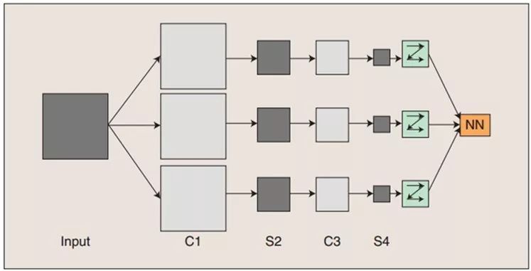
The concept demonstration of convolutional neural networks: input images undergo convolution with three trainable filters and an additive bias, as illustrated in the first figure. After convolution, three feature maps are produced in layer C1, then each group of four pixels in the feature maps is summed, weighted, and biased, and passed through a Sigmoid function to obtain three feature maps in layer S2. These maps are then filtered to produce layer C3. This hierarchical structure also produces S4 just like S2. Finally, these pixel values are rasterized and connected into a vector input to traditional neural networks to obtain output.
In general, the C layer is the feature extraction layer, where each neuron’s input is connected to the local receptive field of the previous layer, extracting features from that local area. Once the local features are extracted, the positional relationships with other features are also determined; the S layer is the feature mapping layer, where each computation layer of the network consists of multiple feature maps, each feature map being a plane with equal weights for all neurons. The feature mapping structure uses a small influence function kernel sigmoid function as the activation function for the convolutional network, ensuring that the feature mapping has translation invariance.
Additionally, since the neurons on a mapping surface share weights, the number of free parameters in the network is reduced, simplifying the complexity of parameter selection. Each feature extraction layer (C-layer) in convolutional neural networks is followed by a computational layer (S-layer) for local averaging and secondary extraction; this unique two-stage feature extraction structure gives the network a high tolerance for distortions in input samples during recognition.
The Training Process of Convolutional Neural Networks
Neural networks used for pattern recognition predominantly employ supervised learning networks, while unsupervised learning networks are more often used for clustering analysis. For supervised pattern recognition, since the category of each sample is known, the distribution of samples in space is no longer divided according to their natural distribution tendencies, but rather seeks an appropriate spatial division method based on the distribution of similar samples in space and the separation degree between different samples, or finds a classification boundary that places different class samples in separate regions. This requires a long and complex learning process, continuously adjusting the position of the classification boundary used to divide the sample space, ensuring that as few samples as possible are classified into non-similar regions.
Convolutional networks are essentially a mapping from input to output, capable of learning a large number of mappings between inputs and outputs without requiring any precise mathematical expressions between inputs and outputs. As long as the convolutional network is trained with known patterns, it gains the ability to map between input and output pairs. Convolutional networks are trained in a supervised manner, so their sample set consists of vector pairs of the form (input vector, ideal output vector). All these vector pairs should originate from the actual “running” results of the system that the network is about to simulate. They can be collected from the actual running system. Before starting the training, all weights should be initialized with different small random numbers. “Small random numbers” ensure that the network does not enter a saturation state due to excessively large weights, leading to training failure; “different” ensures that the network can learn normally. In fact, if the same number is used to initialize the weight matrix, the network will have no capacity to learn.
The training algorithm is similar to the traditional BP algorithm. It mainly includes four steps, divided into two phases:
First phase, forward propagation phase:
a) Take a sample (X,Yp) from the sample set and input X into the network;
b) Calculate the corresponding actual output Op.
In this phase, information is transmitted from the input layer through successive transformations to the output layer. This process is also executed when the network operates normally after training. During this process, the network performs calculations (essentially multiplying the input with the weight matrix of each layer to obtain the final output): Op=Fn(…(F2(F1(XpW(1))W(2))…)W(n))
Second phase, backward propagation phase:
a) Calculate the difference between the actual output Op and the corresponding ideal output Yp;
b) Adjust the weight matrix based on the method of minimizing the error through backpropagation.
Advantages of Convolutional Neural Networks
Convolutional Neural Networks (CNNs) are mainly used to recognize two-dimensional graphics that are invariant to translation, scaling, and other forms of distortion. Because the feature detection layer of CNNs learns through training data, explicit feature extraction is avoided, implicitly learning from the training data. Furthermore, since the weights of neurons on the same feature mapping surface are the same, the network can learn in parallel, which is a significant advantage of convolutional networks over networks where neurons are interconnected. Convolutional Neural Networks have unique advantages in speech recognition and image processing due to their local weight-sharing structure, which closely resembles actual biological neural networks, reducing the complexity of the network, especially the feature extraction and classification processes where multi-dimensional input vectors (images) can be directly input into the network.
The classification methods of the flow are almost all based on statistical features, which means that certain features must be extracted before distinguishing. However, explicit feature extraction is not easy and is not always reliable in some application problems. Convolutional Neural Networks avoid explicit feature sampling, learning implicitly from training data. This makes CNNs significantly different from other neural network-based classifiers, integrating feature extraction functions into multi-layer perceptrons through structural reorganization and reduced weights. It can directly process grayscale images and is suitable for image-based classification.
Convolutional networks have the following advantages over general neural networks in image processing:
a) The input images and the network topology fit well;
b) Feature extraction and pattern classification occur simultaneously, generating both during training;
c) Weight sharing can reduce the training parameters of the network, simplifying the neural network structure and enhancing adaptability.
For submissions, please click “Read the Original”

Reviewed by: Li Guoqing
Source: Sensor Technology, if there are any copyright issues, please contact us in time, the interpretation of copyright belongs to the original author, this article is recommended for reading by Intelligent Manufacturing IMS!