
Deep learning, also known as Deep Learning, is a learning algorithm and an important branch of artificial intelligence. In just a few years, deep learning has revolutionized algorithm design in various fields such as speech recognition, image classification, and text understanding, gradually forming a new model that starts from training data, goes through an end-to-end model, and directly outputs the final result. So, how deep is deep learning? How much can we learn from it? This article will guide you through the methods and processes behind the high-end style of deep learning.
1. Overview
Artificial Intelligence, like immortality and interstellar travel, is one of humanity’s greatest dreams. Although computer technology has made significant progress, no computer has yet produced self-awareness. Yes, with the help of humans and a wealth of existing data, computers can perform impressively, but without these two, they cannot even distinguish between a cat and a dog.
Alan Turing (you all know him, right? The father of computers and artificial intelligence, corresponding to his famous “Turing Machine” and “Turing Test”) proposed the idea of the Turing Test in a 1950 paper, suggesting a conversation behind a wall where you would not know whether you were talking to a person or a computer. This undoubtedly set a high expectation for computers, especially artificial intelligence. However, half a century later, the progress of artificial intelligence has not met the standards of the Turing Test, leading many who have been eagerly waiting to feel disheartened, thinking artificial intelligence is a hoax and related fields are “pseudoscience.”
However, since 2006, the field of machine learning has made groundbreaking progress. The Turing Test is at least not so unattainable anymore. As for the technical means, it relies not only on the parallel processing capabilities of cloud computing on big data but also on algorithms. This algorithm is Deep Learning. With the help of Deep Learning algorithms, humanity has finally found a way to tackle the age-old problem of processing “abstract concepts.”
In June 2012, The New York Times revealed the Google Brain project, attracting widespread public attention. This project, led by renowned Stanford University machine learning professor Andrew Ng and world-class expert Jeff Dean in large-scale computer systems, trained a machine learning model called “Deep Neural Networks” (DNN) on a parallel computing platform with 16,000 CPU cores (internally comprising 1 billion nodes). This network is naturally incomparable to the human neural network, which has over 150 billion neurons and trillions of synapses. It has been estimated that if all the axons and dendrites of all neurons in a human brain were connected in a straight line, it could reach the moon and back to Earth.
One of the project leaders, Andrew, stated: “We didn’t constrain boundaries as we usually do, but directly fed massive amounts of data into the algorithm and let the data speak for itself; the system learns automatically from the data.” Another leader, Jeff, said: “We never tell the machine, ‘This is a cat.’ The system actually invents or understands the concept of ‘cat’ on its own.”
In November 2012, Microsoft publicly demonstrated a fully automated simultaneous interpretation system at an event in Tianjin, China, where the speaker delivered a speech in English, and the computer seamlessly completed speech recognition, English-Chinese machine translation, and Chinese speech synthesis in the background, achieving very smooth results. According to reports, the key technology supporting this was also DNN or Deep Learning.
In January 2013, at Baidu’s annual meeting, founder and CEO Li Yanhong announced the establishment of Baidu Research Institute, with the first established being the “Institute of Deep Learning” (IDL).
Why are internet companies with big data scrambling to invest substantial resources in deep learning technology? It sounds like deep learning is very powerful. So what is deep learning? Why do we have deep learning? How did it come about? What can it do? What difficulties currently exist? These questions require detailed discussion. Let’s first understand the background of machine learning, the core of artificial intelligence.
2. Background
Machine Learning is a discipline that specializes in studying how computers can simulate or implement human learning behavior to acquire new knowledge or skills and reorganize existing knowledge structures to continuously improve their performance. Can machines learn like humans? In 1959, Samuel from the United States designed a chess program that had learning capabilities, allowing it to improve its chess skills through continuous games. Four years later, this program defeated its creator. Three years later, it defeated a champion who had maintained an undefeated record for eight years. This program demonstrated the power of machine learning and raised many thought-provoking social and philosophical questions.
Although machine learning has developed over several decades, many unresolved issues remain:
For example, image recognition, speech recognition, natural language understanding, weather prediction, gene expression, content recommendation, etc. Currently, our approach to solving these problems through machine learning is as follows (taking visual perception as an example):
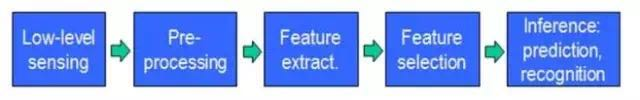
Starting by obtaining data through sensors (e.g., CMOS), then preprocessing, feature extraction, feature selection, and finally reasoning, predicting, or recognizing. The last part, which is the machine learning part, involves most of the work done here, and many papers and research exist in this area.
The middle three parts can be summarized as feature representation. Good feature representation plays a crucial role in the accuracy of the final algorithm, and most of the system’s computation and testing work is consumed in this large part. However, this part is generally completed manually in practice, relying on manual feature extraction.
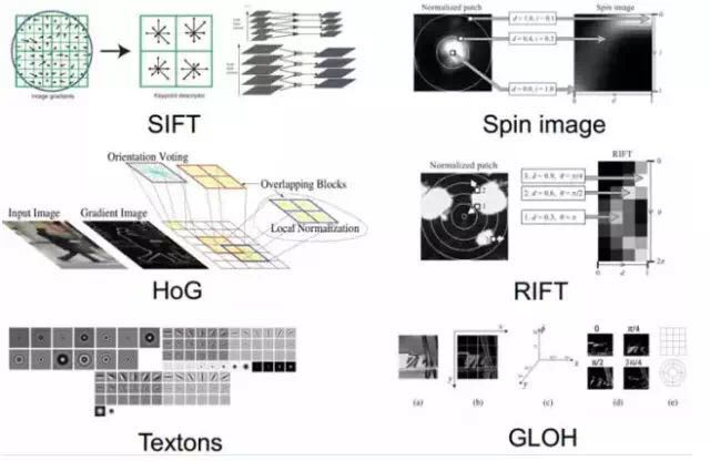
As of now, many excellent features have emerged (good features should have invariance to size, scale, rotation, etc., and distinguishability): for example, the emergence of SIFT is a milestone in the study of local image feature descriptors. Because SIFT is invariant to scale, rotation, and certain variations in perspective and lighting, it indeed makes the solution of many problems possible. But it is not a panacea.
However, manually selecting features is a very labor-intensive and heuristic method, which largely depends on experience and luck, and its adjustment requires a lot of time. Since manual feature selection is not ideal, can we automatically learn some features? The answer is yes! Deep Learning is used for this purpose, as its other name, Unsupervised Feature Learning, implies that it does not require human involvement in the feature selection process.
So how does it learn? How does it know which features are good and which are not? We say machine learning is a discipline that specializes in studying how computers can simulate or implement human learning behavior. Well, how does our visual system work? Why can we find another person in the vast sea of humanity? (Because you exist in my deep memory, in my dreams, in my heart, in my song…) Our brains are so remarkable; can we refer to them and simulate them? (It seems that features and algorithms related to the human brain are good, but who knows if they are artificially imposed to make their works seem sacred and elegant.) In recent decades, the development of cognitive neuroscience, biology, and other disciplines has made us less unfamiliar with our mysterious and magical brains, and has also propelled the development of artificial intelligence.
3. Human Visual Processing
The Nobel Prize in Physiology or Medicine in 1981 was awarded to David Hubel (a Canadian-American neurobiologist) and Torsten Wiesel, as well as Roger Sperry. The main contribution of the first two was the “discovery of information processing in the visual system”: the visual cortex is hierarchical:
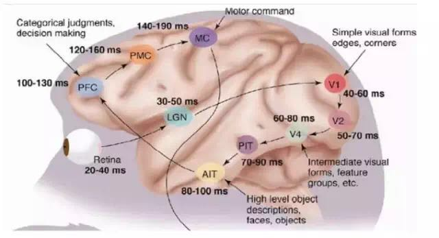
Let’s take a look at what they did. In 1958, David Hubel and Torsten Wiesel at Johns Hopkins University studied the correspondence between pupil regions and cortical neurons. They made a 3 mm hole in the skull of a cat and inserted electrodes to measure the activity of neurons.
Then, they presented various shapes and brightness levels of objects in front of the kitten. Moreover, they changed the position and angle of the objects during the presentation. They hoped to use this method to let the kitten’s pupil perceive different types and strengths of stimuli.
The purpose of this experiment was to prove a hypothesis: that different visual neurons in the posterior cortex correspond to the stimuli received by the pupil. Once the pupil is stimulated by a certain type of stimulus, a specific part of the posterior cortex’s neurons will become active. After many days of repetitive and tedious experiments, and the sacrifice of several unfortunate kittens, David Hubel and Torsten Wiesel discovered a type of neuron called “Orientation Selective Cell.” When the pupil detects the edge of an object in front of it, and this edge points in a certain direction, this type of neuron will become active.
This discovery sparked further thinking about the nervous system. The working process of the nervous-central-brain may be a continuous iteration and abstraction process. Here, two keywords are important: abstraction and iteration. From raw signals, low-level abstractions are made, gradually iterating towards high-level abstractions. Human logical thinking often uses highly abstract concepts.
For example, starting from the raw signal intake (the pupil receives pixel data), then performing preliminary processing (certain cells in the brain detect edges and directions), followed by abstraction (the brain determines that the shape of the object in front is circular), and further abstraction (the brain further determines that the object is a balloon).
This physiological discovery facilitated the breakthrough development of artificial intelligence four decades later.
In summary, the information processing of the human visual system is hierarchical. From low-level V1 area extracting edge features, to V2 area recognizing shapes or parts of objects, to higher levels recognizing entire objects and their behaviors. In other words, high-level features are combinations of low-level features, and feature representation becomes increasingly abstract and able to express semantics or intentions. The higher the abstraction level, the fewer possible guesses exist, making classification easier. For example, the correspondence between a set of words and sentences is many-to-one, and the correspondence between sentences and semantics is also many-to-one, as is the correspondence between semantics and intentions; this forms a hierarchical system.
Sensitive individuals have noticed the keywords: hierarchy. And does the “deep” in deep learning indicate how many layers I have, or how deep it is? That’s right. So how does deep learning borrow from this process? After all, it is a computer processing task, and the challenge is how to model this process.
Since we need to learn feature representation, we need to delve deeper into the features or the hierarchical features. Therefore, before discussing deep learning, it is necessary to elaborate on features (actually, it seems a bit regrettable not to include such good explanations about features here, so I will add it here).
4. About Features
Features are the raw materials of machine learning systems, and their influence on the final model is unquestionable. If data is well expressed as features, linear models can usually achieve satisfactory accuracy. So what should we consider for features?
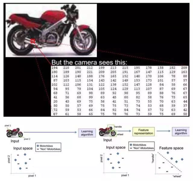
4.1. The Granularity of Feature Representation
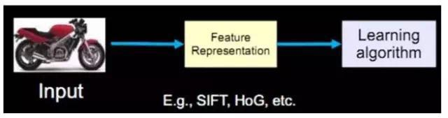
At what granularity should the learning algorithm represent features to be effective? For example, for an image, pixel-level features are of no value. For instance, the motorcycle below cannot be distinguished between a motorcycle and a non-motorcycle at the pixel level. However, if the feature has a structure (or meaning), such as whether it has handlebars or wheels, it becomes easy to distinguish between a motorcycle and a non-motorcycle, allowing the learning algorithm to function.
4.2. Primary (Shallow) Feature Representation
Since pixel-level feature representation methods are ineffective, what kind of representation is useful?
In the mid-1990s, scholars Bruno Olshausen and David Field at Cornell University attempted to study visual problems using both physiological and computational methods. They collected many black-and-white landscape photos and extracted 400 small fragments, each measuring 16×16 pixels, which we can label as S[i], i = 0,…, 399. Next, they randomly selected another fragment from these black-and-white landscape photos, also measuring 16×16 pixels, which we can label as T.
The question they posed was how to select a set of fragments, S[k], from these 400 fragments to combine them to create a new fragment that should be as similar as possible to the randomly selected target fragment T, while minimizing the number of S[k]. Mathematically, this can be described as:
*Sum_k (a[k] * S[k]) –> T, where a[k] is the weight coefficient when combining fragments S[k].
To solve this problem, Bruno Olshausen and David Field invented an algorithm called Sparse Coding. Sparse coding is a repetitive iterative process with two steps for each iteration:
*1) Select a set of S[k] and adjust a[k] to make Sum_k (a[k] * S[k]) as close to T as possible.
*2) Fix a[k] and choose other more suitable fragments S'[k] from the 400 fragments to replace the original S[k], making Sum_k (a[k] * S'[k]) as close to T as possible.
After several iterations, the best S[k] combination is selected. Amazingly, the selected S[k] are primarily edge lines of different objects in the photos, with similar shapes but differing in direction. The results of Bruno Olshausen and David Field’s algorithm coincided with the physiological findings of David Hubel and Torsten Wiesel!
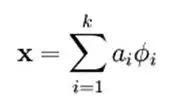
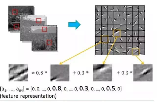
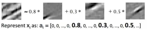
In other words, complex patterns are often composed of some basic structures. For example, the following diagram shows that a figure can be linearly represented by 64 orthogonal edges (which can be understood as orthogonal basic structures). For instance, the sample x can be formed by blending three of the 64 edges with weights of 0.8, 0.3, and 0.5, while the other basic edges contribute nothing and are thus zero.
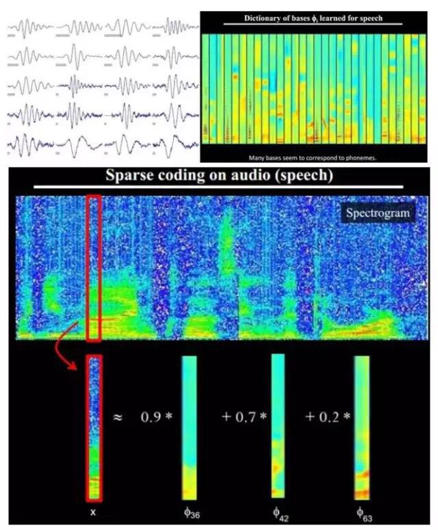
Additionally, researchers have discovered that this pattern exists not only in images but also in sounds. They found 20 basic sound structures from unlabeled sounds, and the remaining sounds could be composed of these 20 basic structures.
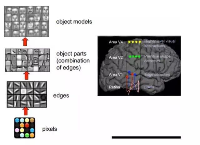
4.3. Structured Feature Representation
Small graphical pieces can be constructed from basic edges; how can more structured and complex conceptual graphics be represented? This requires higher-level feature representation, such as V2 and V4. Therefore, V1 looks at pixel-level features, while V2 looks at V1 as pixel-level; this is a hierarchical progression, where high-level expressions are combinations of low-level expressions. More professionally speaking, these are basis functions. The basis proposed by V1 is edges, while the V2 layer is a combination of these V1 basis functions; at this point, the V2 area obtains a higher-level basis. In other words, the results of combining the previous layer’s basis yield the next layer’s basis… (This is why some experts say deep learning is about “basis”, which sounds unpleasant, so it’s elegantly named Deep Learning or Unsupervised Feature Learning.)
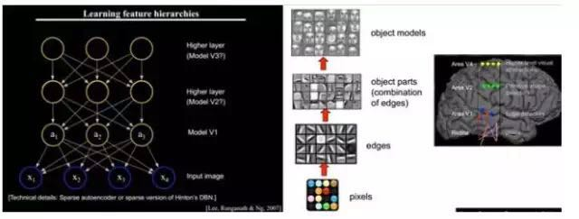
Intuitively, it’s about finding meaningful small patches and combining them to obtain the previous layer’s features, recursively learning features upward.
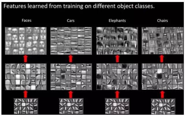
When training on different objects, the obtained edge basis is very similar, but the object parts and models will be completely different (making it much easier for us to distinguish between cars or faces):
From a textual perspective, how does a document convey meaning? What is the most appropriate way to describe an event? Using individual words? I don’t think so; words are at the pixel level. At the very least, it should be at the term level, meaning each document consists of terms, but is that enough to represent the concept? Perhaps not; we may need to go one step further to the topic level. Once we have a topic, it becomes reasonable to connect it back to the document. However, the quantity differences at each level are significant, for example, the correspondence between document representations and topics is on the order of thousands to tens of thousands, while terms are on the order of hundreds of thousands, and words are on the order of millions.
When a person reads a document, their eyes see words, and these words automatically segment into terms in the brain, organized according to concepts, leading to prior learning to obtain topics, followed by higher-level learning.
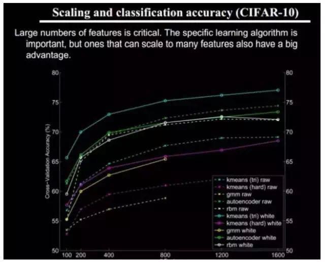
4.4. How Many Features Are Needed?
We know that hierarchical feature construction is required, progressing from shallow to deep, but how many features should each layer have?
In any method, the more features there are, the more reference information is provided, which can improve accuracy. However, having too many features means increased computational complexity, larger exploration space, and sparsity of training data for each feature, which can lead to various problems; more features do not necessarily mean better outcomes.
Alright, at this point, we can finally talk about deep learning. We discussed why deep learning exists (to allow machines to automatically learn good features without manual selection, and to refer to the hierarchical visual processing system of humans), and we conclude that deep learning requires multiple layers to obtain more abstract feature representations. So how many layers are appropriate? What architecture should be used for modeling? How is unsupervised training conducted?
5. Basic Ideas of Deep Learning
Suppose we have a system S with n layers (S1,…Sn), its input is I, and its output is O, which can be visually represented as: I =>S1=>S2=>…..=>Sn => O. If the output O is equal to the input I, meaning that the input I undergoes no information loss after passing through this system (Haha, experts say this is impossible. In information theory, there is a saying about “information loss at each layer” (information processing inequality), which states that if processing information a results in b, and then processing b results in c, it can be proven that the mutual information between a and c will not exceed the mutual information between a and b. This indicates that information processing does not increase information; most processing results in information loss. Of course, if the lost information is useless, that would be great.), it means that the input I is another representation of the original information (i.e., input I) at every layer Si. Now returning to our topic of deep learning, we need to automatically learn features. Suppose we have a bunch of inputs I (like a set of images or texts), and assume we design a system S (with n layers), we can adjust the parameters in the system so that its output is still the input I, and then we can automatically obtain a series of hierarchical features of input I, namely S1, …, Sn.
For deep learning, the idea is to stack multiple layers, meaning that the output of one layer serves as the input to the next layer. Through this approach, we can achieve a hierarchical expression of input information.
Moreover, the previous assumption that output strictly equals input is too strict; we can relax this condition slightly, for example, we only need to make the difference between input and output as small as possible. This relaxation leads to another type of deep learning method. The above describes the basic ideas of deep learning.
6. Shallow Learning and Deep Learning
Shallow learning is the first wave of machine learning.
In the late 1980s, the invention of the backpropagation algorithm (also known as the BP algorithm) for artificial neural networks brought hope to machine learning and sparked a wave of machine learning based on statistical models that continues to this day. People discovered that using the BP algorithm allows an artificial neural network model to learn statistical rules from a large number of training samples and predict unknown events. This statistical-based machine learning method shows superiority in many aspects compared to previous systems based on artificial rules. At this time, artificial neural networks, although also known as multi-layer perceptrons, are essentially shallow models containing only one hidden layer.
In the 1990s, various shallow machine learning models were proposed, such as Support Vector Machines (SVM), Boosting, and Maximum Entropy methods (like Logistic Regression). The structures of these models can generally be seen as having one layer of hidden nodes (like SVM, Boosting) or no hidden nodes (like Logistic Regression). These models have achieved great success in both theoretical analysis and applications. In contrast, due to the difficulty of theoretical analysis and the need for much experience and skill in training methods, shallow artificial neural networks became relatively quiet during this period.
Deep learning represents the second wave of machine learning.
In 2006, Geoffrey Hinton, a professor at the University of Toronto and a leader in the field of machine learning, along with his student Ruslan Salakhutdinov, published a paper in Science that ignited a wave of deep learning in academia and industry. This paper made two main points: 1) Multi-hidden-layer artificial neural networks have excellent feature learning capabilities, and the features learned provide a more essential characterization of the data, facilitating visualization or classification; 2) The training difficulty of deep neural networks can be effectively overcome through “layer-wise pre-training”; in this paper, layer-wise pre-training is achieved through unsupervised learning.
Currently, most classification, regression, and other learning methods are shallow structure algorithms, which are limited by their ability to represent complex functions under conditions of limited samples and computational units, and their generalization ability is constrained for complex classification problems. Deep learning can learn a deep non-linear network structure to approximate complex functions, represent the distributed representation of input data, and show strong capabilities to learn the essential features of datasets from a small number of samples. (The advantage of multiple layers is that they can represent complex functions with fewer parameters.)

Deep learning’s essence is to construct machine learning models with many hidden layers and vast amounts of training data to learn more useful features, ultimately improving classification or prediction accuracy. Therefore, “deep models” are the means, while “feature learning” is the goal. In contrast to traditional shallow learning, the difference in deep learning is: 1) It emphasizes the depth of the model structure, usually having 5, 6, or even more than 10 hidden layers; 2) It explicitly highlights the importance of feature learning, meaning that through layer-wise feature transformations, the representation of samples in the original feature space is transformed into a new feature space, making classification or prediction easier. Compared to the manual rule-based feature construction methods, using big data to learn features can better characterize the rich intrinsic information of the data.
7. Deep Learning and Neural Networks
Deep learning is a new area of research in machine learning, motivated by the establishment and simulation of neural networks that analyze and learn like the human brain, mimicking the mechanisms of the brain to interpret data such as images, sounds, and text. Deep learning is a form of unsupervised learning.
The concept of deep learning originates from the study of artificial neural networks. Multi-layer perceptrons with multiple hidden layers are a form of deep learning structure. Deep learning combines low-level features to form more abstract high-level representations of attribute categories or features, discovering distributed feature representations of data.
Deep learning can be considered a branch of machine learning, which can be simply understood as the development of neural networks. About 20 to 30 years ago, neural networks were a particularly hot direction in the field of machine learning, but gradually faded away for several reasons:
1) They are prone to overfitting, parameters are difficult to tune, and require many tricks;
2) Training speed is slow, and in cases with fewer layers (less than or equal to 3), their performance is not superior to other methods;
Thus, for about 20 years, neural networks received little attention, and this period was essentially dominated by SVM and boosting algorithms. However, one dedicated old gentleman, Hinton, persisted and eventually (along with others like Bengio, Yann LeCun, etc.) proposed a practically feasible deep learning framework.
Deep learning and traditional neural networks share similarities but also have many differences.
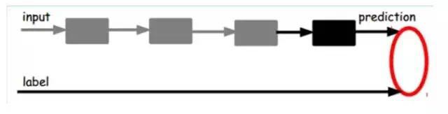
Both adopt a similar hierarchical structure, where the system consists of an input layer, hidden layers (multiple layers), and an output layer. Only adjacent layer nodes are connected, while there are no connections within the same layer or across layers. Each layer can be viewed as a logistic regression model; this hierarchical structure closely resembles the structure of the human brain.
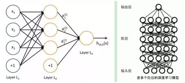
To overcome the issues in training neural networks, deep learning employs a training mechanism that differs significantly from traditional neural networks. In traditional neural networks, the backpropagation method is used for training, which can be simply described as an iterative algorithm to train the entire network, randomly setting initial values, calculating the current network output, and then adjusting the parameters of the previous layers based on the difference between the current output and the label until convergence (the overall process is a gradient descent method). In contrast, deep learning employs a layer-wise training mechanism. The reason for this is that if the backpropagation mechanism is used for a deep network (more than 7 layers), the residuals that propagate back to the earlier layers become too small, leading to the so-called gradient diffusion. We will discuss this problem next.
8. Training Process of Deep Learning
8.1. Why Traditional Neural Network Training Methods Cannot Be Used in Deep Neural Networks
As a typical algorithm for training multi-layer networks, the BP algorithm is already not ideal for networks with only a few layers. The presence of local minima in non-convex objective cost functions in deep structures (involving multiple non-linear processing unit layers) is the main source of training difficulties.
Problems with the BP algorithm include:
(1) Gradients become increasingly sparse: as you go deeper from the top layer, the error correction signals become smaller;
(2) Convergence to local minima: especially when starting far from the optimal area (random initialization can lead to this situation);
(3) Generally, we can only train using labeled data: but most data is unlabeled, whereas the brain can learn from unlabeled data;
8.2. The Deep Learning Training Process
If all layers are trained simultaneously, the time complexity will be too high; if each layer is trained one at a time, the bias will propagate layer by layer. This faces the opposite problem compared to supervised learning, leading to severe underfitting (because deep networks have too many neurons and parameters).
In 2006, Hinton proposed an effective method for establishing multi-layer neural networks on unlabeled data, simply put, divided into two steps: first, train one layer of the network at a time, and second, tune the parameters such that the high-level representation generated from the original representation x and the high-level representation r is as consistent as possible with the original representation x. The method is:
1) First, build single-layer neurons layer by layer, training one single-layer network each time.
2) Once all layers are trained, Hinton uses the wake-sleep algorithm for tuning.
This method turns the weights between all layers except the top layer into bidirectional weights, while the top layer remains a single-layer neural network, and the other layers become graphical models. The upward weights are used for “cognition,” and the downward weights are used for “generation.” Then, the Wake-Sleep algorithm adjusts all the weights. The goal is to ensure that the generated top-level representation can accurately restore the bottom layer nodes. For example, if a node at the top level represents a face, then all images of faces should activate this node, and the resulting image generated should represent a rough face image.
The wake-sleep algorithm consists of two parts:
**1) Wake phase:** the cognitive process generates abstract representations (node states) for each layer through external features and upward weights (cognitive weights), while using gradient descent to modify the downward weights (generative weights). In other words, “If reality differs from my imagination, I will change my weights to make my imagination match reality.”
**2) Sleep phase:** the generative process generates bottom-layer states through the top-level representation (the concepts learned during wake) and downward weights, while modifying the upward weights. In other words, “If the scenes in my dreams do not match the corresponding concepts in my mind, I will change my cognitive weights to make the scene appear to me as that concept.”
The specific training process for deep learning is as follows:
1) Use bottom-up unsupervised learning (i.e., training layer by layer from the bottom up):
Using unlabeled data (labeled data can also be used), train the parameters of each layer, which can be seen as an unsupervised training process. This step is the largest difference from traditional neural networks (this process can be considered as feature learning).
Specifically, first train the first layer with unlabeled data, learning the parameters of the first layer (this layer can be seen as obtaining a hidden layer of a three-layer neural network that minimizes the difference between input and output). Due to model capacity limitations and sparsity constraints, the resulting model can learn the structure of the data itself, obtaining features with greater representational capacity than the input. After learning the n-1 layer, the output of the n-1 layer is used as the input for the n-th layer, and the n-th layer is trained, thus obtaining the parameters for each layer;
2) Top-down supervised learning (i.e., training with labeled data, transmitting errors from top to bottom, fine-tuning the network):
Based on the parameters obtained from the first step, further fine-tune the parameters of the entire multi-layer model through supervised training; this step is a supervised training process. The first step is similar to the random initialization process in neural networks, but since the first step of deep learning is not random initialization, but rather learning the structure of the input data, this initial value is closer to the global optimal, thus achieving better results. Therefore, much of the effectiveness of deep learning can be attributed to the feature learning process in the first step.
9. Common Models or Methods in Deep Learning
9.1. AutoEncoder
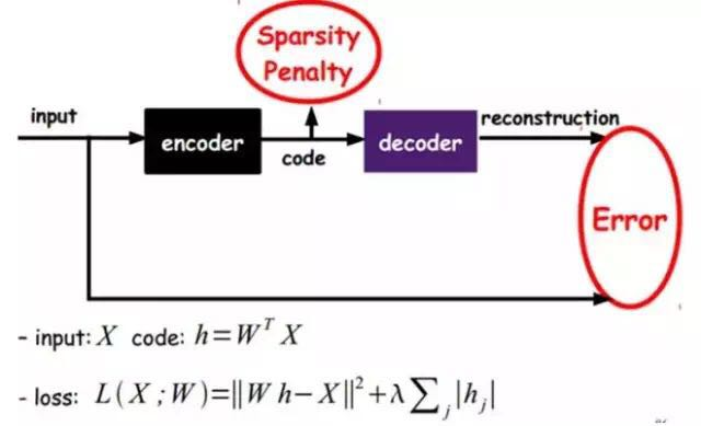
The simplest method in deep learning is to utilize the characteristics of artificial neural networks. Artificial Neural Networks (ANNs) themselves are systems with hierarchical structures. If a neural network is given, we assume that its output is the same as its input, and then train to adjust its parameters to obtain the weights in each layer. Naturally, we obtain several different representations of the input I (each layer represents a representation); the autoencoder is a neural network that aims to reproduce the input signal as closely as possible. To achieve this reproduction, the autoencoder must capture the most important factors that can represent the input data, similar to PCA, finding the main components that can represent the original information.
The specific process can be briefly described as follows:
1) Given unlabeled data, learn features through unsupervised learning:
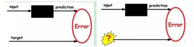
In our previous neural network, the input samples were labeled (i.e., (input, target)), so we adjusted the parameters of the previous layers based on the difference between the current output and the target until convergence. But now we only have unlabeled data, which means we do not have a target. So how do we obtain the error?
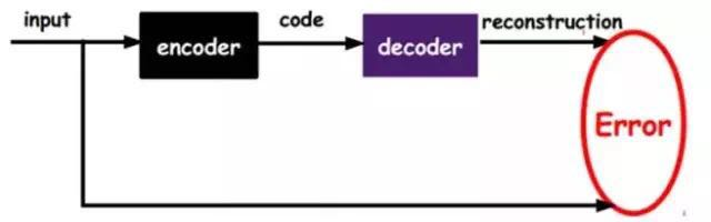
As shown in the above diagram, we input the input into an encoder, which will produce a code; this code is a representation of the input. How do we know this code is representative of the input? We add a decoder, which will output information, and if this output is very similar to the initial input signal (ideally, the same), then we have reason to believe that this code is reliable. Therefore, we adjust the parameters of the encoder and decoder to minimize the reconstruction error; at this point, we obtain the first representation of the input signal, which is the encoded code. Since it is unlabeled data, the source of the error is directly the comparison between the reconstruction and the original input.
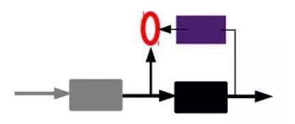
2) Generate features through the encoder, then train the next layer. Train layer by layer:
At this point, we have obtained the first layer’s code, and minimizing the reconstruction error allows us to believe that this code is a good representation of the original input signal (or, to put it somewhat forcedly, it is exactly the same). The second layer’s training is no different from the first layer’s: we take the output of the first layer as the input signal for the second layer, minimizing the reconstruction error again to obtain the parameters for the second layer and the code for the second layer’s input, which is the second representation of the original input information. The same method can be applied to subsequent layers (training this layer while fixing the parameters of the previous layers, and the decoders are no longer needed).
3) Supervised fine-tuning:
After the above methods, we can obtain many layers. As for how many layers (or how deep is appropriate), there is currently no scientific evaluation method; it requires experimentation. Each layer will obtain a different representation of the original input. Of course, we believe that the more abstract, the better, just like the human visual system.
At this point, the autoencoder cannot yet be used for classifying data, as it has not yet learned how to connect an input to a class. It has only learned how to reconstruct or reproduce its input. In other words, it has only learned to obtain a feature that can best represent the input signal. Therefore, in order to achieve classification, we can add a classifier (such as logistic regression, SVM, etc.) at the topmost encoding layer of the autoencoder and then train it using standard supervised training methods for multi-layer neural networks (gradient descent method).
In other words, at this point, we need to input the feature code from the last layer into the final classifier and fine-tune it through supervised learning using labeled samples, which can be done in two ways: one is to only adjust the classifier (the black part):
The other is to fine-tune the entire system with labeled samples (if there is enough data, this is the best. End-to-end learning):
Once the supervised training is completed, this network can be used for classification. The top layer of the neural network can serve as a linear classifier, and we can replace it with a higher-performing classifier. Research has shown that incorporating these automatically learned features into the original features can significantly improve accuracy, even outperforming the best classification algorithms currently available!
Autoencoders have some variants; here are brief introductions to two:
Sparse AutoEncoder:
Of course, we can also add some constraints to obtain new deep learning methods. For example, if we add an L1 Regularization constraint to the AutoEncoder (L1 mainly constrains that most nodes in each layer must be zero, with only a few being non-zero, which is the origin of the name Sparse), we can obtain the Sparse AutoEncoder method.
As shown in the above diagram, this method aims to ensure that the expression code obtained each time is as sparse as possible. This is because sparse representations are often more effective than other representations (the human brain seems to work similarly, where a certain input only stimulates certain neurons, while the majority of neurons are inhibited).
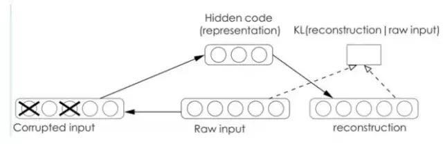
Denoising AutoEncoders:
Denoising AutoEncoder (DA) is based on the AutoEncoder, where noise is added to the training data, forcing the autoencoder to learn to remove this noise to obtain the true input that has not been polluted by noise. Therefore, this compels the encoder to learn a more robust representation of the input signal, which is also why its generalization ability is stronger than that of a typical encoder. DA can be trained using the gradient descent algorithm.
9.2. Sparse Coding
Φ1 + a2undefined_Φ2+….+ an*Φn, where Φi is the basis and ai is the coefficient, we can obtain the following optimization problem:
Min |I – O|, where I represents input and O represents output.
By solving this optimization equation, we can find the coefficients ai and bases Φi, which serve as another approximate representation of the input.
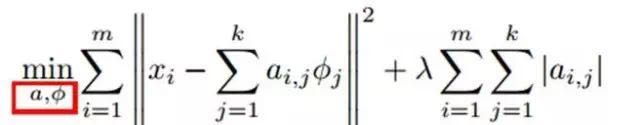
Therefore, they can be used to express input I, and this process is also learned automatically. If we add an L1 Regularization constraint to the above equation, we get:
Min |I – O| + u*(|a1| + |a2| + … + |an |)
This method is called Sparse Coding. Simply put, it represents a signal as a linear combination of a set of bases while requiring that only a few bases are needed to represent the signal. “Sparsity” is defined as having only a few non-zero elements or only a few significantly larger than zero elements. The requirement for coefficients ai to be sparse means that for a set of input vectors, we want as few coefficients as possible to be significantly greater than zero. The reason for choosing to use components with sparsity to represent our input data is that the vast majority of sensory data, such as natural images, can be represented as the sum of a few basic elements. In images, these basic elements can be edges or lines. Additionally, the analogy to the process of the primary visual cortex has been enhanced (the human brain has a large number of neurons, but for certain images or edges, only a few neurons become excited while the rest remain inhibited).
Sparse coding algorithms are a form of unsupervised learning that seeks a set of “overcomplete” basis vectors to represent sample data more efficiently. Although techniques like Principal Component Analysis (PCA) can easily find a set of “complete” basis vectors, what we want to do here is find a set of “overcomplete” basis vectors to represent the input vector (meaning that the number of basis vectors exceeds the dimensionality of the input vector). The advantage of overcomplete bases is that they can more effectively identify the structures and patterns hidden within the input data. However, for overcomplete bases, coefficients ai are no longer uniquely determined by the input vector. Therefore, in sparse coding algorithms, we add a criterion of “sparsity” to address the degeneracy issue caused by overcompleteness.
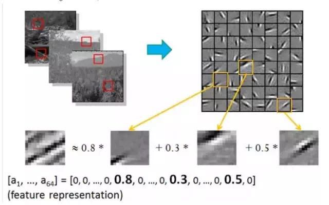
For instance, when generating edge detectors at the lowest level of image feature extraction, the work involves randomly selecting small patches from natural images and generating the “basis” that can describe them, as shown on the right, which consists of 64 basis functions. Given a test patch, we can use the basis linear combination to obtain it, with the sparse matrix being a, where the matrix a has 64 dimensions, with only three non-zero entries, hence the term “sparse.”
Here, you may wonder why the lowest level is considered an edge detector. What about the upper layers? A simple explanation is that different directional edges can describe the entire image, so different directional edges naturally serve as the basis of the image… and the results of the previous layer’s basis combinations yield the next layer’s basis… (as we discussed in the previous section).
Sparse coding consists of two parts:
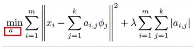
1) Training phase: Given a series of sample images [x1, x2, …], we need to learn a set of bases [Φ1, Φ2, …], which is the dictionary.
Sparse coding is a variant of the k-means algorithm, and its training process is quite similar (following the idea of the EM algorithm: if the objective function to optimize includes two variables, such as L(W, B), we can fix W and adjust B to minimize L, then fix B and adjust W to minimize L, iterating this way to push L towards its minimum value).
The training process is a repetitive iterative process, as described above, where we alternately change a and Φ to minimize the following objective function.
Each iteration consists of two steps:
a) Fix the dictionary Φ[k], then adjust a[k] to minimize the objective function (i.e., solve the LASSO problem).
b) Then fix a[k], adjust Φ[k] to minimize the objective function (i.e., solve the convex quadratic programming problem).
Continue iterating until convergence. This way, we can obtain a set of bases that can effectively represent this series of x, which is the dictionary.
2) Coding phase: Given a new image x, we use the dictionary obtained above to derive a sparse vector a by solving a LASSO problem. This sparse vector is a sparse representation of the input vector x.
For example:
9.3. Restricted Boltzmann Machine (RBM)
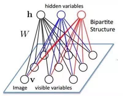
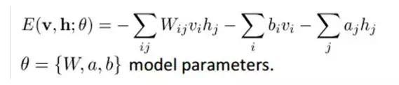
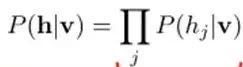
Assume there is a bipartite graph where there are no links between nodes in each layer; one layer is the visible layer, i.e., the input data layer (v), and one layer is the hidden layer (h). If we assume all nodes are random binary variable nodes (can only take values of 0 or 1), and all probability distributions p(v,h) satisfy the Boltzmann distribution, we call this model a Restricted Boltzmann Machine (RBM).

Now let’s see why it is a deep learning method. First, because this model is bipartite, all hidden nodes are conditionally independent given v (because there are no connections between nodes), that is, p(h|v)=p(h1|v)…p(hn|v). Similarly, given the hidden layer h, all visible nodes are conditionally independent. Furthermore, since all v and h satisfy the Boltzmann distribution, when inputting v, we can obtain the hidden layer h through p(h|v), and after obtaining the hidden layer h, we can obtain the visible layer through p(v|h). By adjusting parameters, we aim to make the visible layer obtained from the hidden layer as similar as possible to the original visible layer, thus the hidden layer can serve as another representation of the input data features, making it a deep learning method.

How is it trained? Specifically, how are the weights between the visible layer nodes and hidden nodes determined? We need to conduct some mathematical analysis, which is the model.
The energy of the joint configuration can be expressed as:
The joint probability distribution of a certain configuration can be determined by the Boltzmann distribution (and the energy of that configuration):
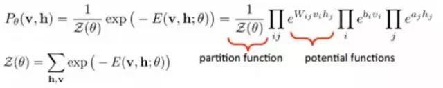
Since the hidden nodes are conditionally independent (because there are no connections between nodes), we have:
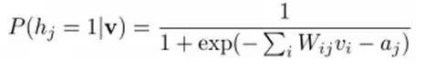
Then we can easily (factorize the above equation) obtain the probability of the j-th hidden layer node being 1 or 0 given the visible layer v:
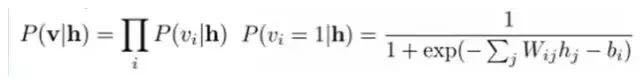
Similarly, based on the hidden layer h, we can easily obtain the probability of the i-th visible layer node being 1 or 0:
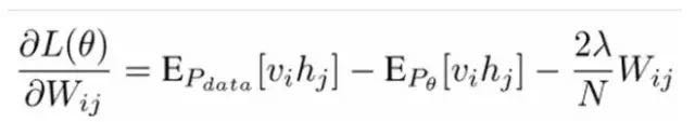
Given a sample set D={v(1), v(2),…, v(N)} that satisfies independent and identically distributed (i.i.d.), we need to learn the parameters θ={W,a,b}.
We maximize the following log-likelihood function (maximum likelihood estimation: for a probability model, we need to choose parameters that maximize the probability of our current observed samples):
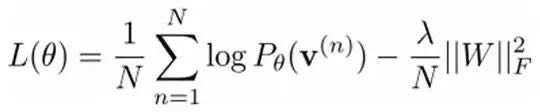
By taking the derivative of the maximum log-likelihood function, we can find the parameters W corresponding to L’s maximum.
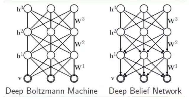
If we increase the number of hidden layers, we can obtain a Deep Boltzmann Machine (DBM). If we use a Bayesian belief network (i.e., a directed graphical model) near the visible layer, while using a Restricted Boltzmann Machine in the farthest part from the visible layer, we can obtain a Deep Belief Network (DBN).
9.4. Deep Belief Networks
DBNs are a probabilistic generative model, in contrast to traditional discriminative models of neural networks. Generative models establish a joint distribution between observed data and labels, assessing both P(Observation|Label) and P(Label|Observation), while discriminative models only assess the latter, namely P(Label|Observation). When applying traditional BP algorithms to deep neural networks, DBNs encounter the following issues:
(1) They require a labeled sample set for training;
(2) The learning process is slow;
(3) Improper parameter selection can lead to learning converging to local optimal solutions.
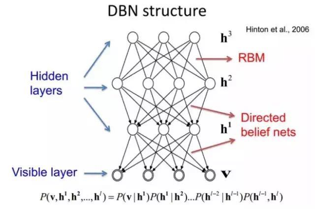
DBNs consist of multiple layers of Restricted Boltzmann Machines (RBMs). A typical neural network structure is shown in the following diagram. These networks are “restricted” to a visible layer and a hidden layer, where connections exist between layers, but there are no connections between units within the same layer. Hidden layer units are trained to capture correlations of high-order data expressed in the visible layer.
Initially, without considering the top two layers that form an associative memory, a DBN’s connections are guided by generative weights from top to bottom, and RBMs serve as building blocks. Compared to traditional and deep layered sigmoid belief networks, it is easier to learn connection weights.
Initially, a greedy layer-wise unsupervised method is used to pre-train and obtain the generative model’s weights, which Hinton has proven to be effective and is referred to as contrastive divergence.
In this training phase, a vector v is produced in the visible layer, passing values to the hidden layer. Conversely, input values in the visible layer are randomly selected to attempt to reconstruct the original input signal. Finally, these new visible neuron activation units will forward transmit to reconstruct hidden layer activation units, obtaining h (during training, the visible vector values are first mapped to hidden units; then visible units are reconstructed by hidden layer units; these new visible units are mapped back to hidden units, thus obtaining new hidden units. This iterative process is called Gibbs sampling). These backward and forward steps are familiar to us from Gibbs sampling, and the difference in correlation between hidden layer activation units and visible layer inputs serves as the primary basis for weight updates.
Training time will be significantly reduced because only a single step is needed to approach maximum likelihood learning. Adding each layer to the network improves the log probability of the training data, which can be understood as getting closer to the true expression of energy. This meaningful expansion and the use of unlabeled data are decisive factors in any deep learning application.
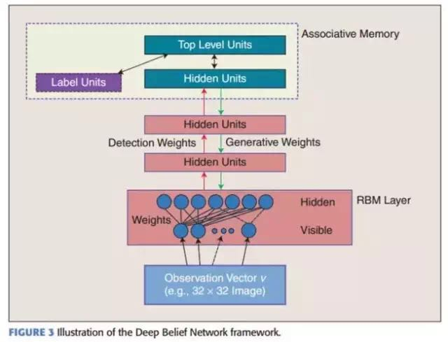
In the top two layers, weights are interconnected, allowing the outputs of lower layers to provide reference clues or associations to the top layer, which in turn links to its memory content. What we are most concerned about is the final discriminative performance, such as in classification tasks.
After pre-training, DBNs can fine-tune their discriminative performance using labeled data with the BP algorithm. In this case, a label set will be attached to the top layer (promoting associative memory), obtaining a classification surface for the network through the learned recognition weights from bottom to top. This performance will be better than that of networks trained solely by the BP algorithm. This can be intuitively explained: the BP algorithm of DBNs only requires local searches in the parameter space, making training faster and reducing convergence time compared to feedforward neural networks.
The flexibility of DBNs makes their expansion relatively easy. One expansion is Convolutional DBNs (CDBNs). DBNs do not consider the two-dimensional structural information of images, as the input is simply vectorized from an image matrix. CDBNs address this issue by utilizing the spatial relationships of neighboring pixels through a model called Convolutional RBMs, achieving translational invariance in generative models and easily transitioning to high-dimensional images. DBNs do not explicitly handle learning the temporal associations of observed variables, although research in this area is ongoing, such as stacking temporal RBMs for sequential learning applications dubbed temporal convolution machines, which bring exciting future research directions for speech signal processing.
Currently, research related to DBNs includes stacked autoencoders, which replace the RBMs in traditional DBNs. This allows for training deep multi-layer neural network architectures using the same rules, but it lacks the strict parameterization requirements of layers. Unlike DBNs, autoencoders use discriminative models, making it more challenging to sample input spaces, which makes it difficult for the network to capture its internal representations. However, denoising autoencoders can effectively avoid this issue and outperform traditional DBNs. They enhance generalization performance by adding random noise during the training process and stacking.
10. Summary and Outlook
1) Summary of Deep Learning
Deep learning is an algorithm about automatically learning the latent (implicit) distribution of data to build complex multi-layer representations. In other words, deep learning algorithms automatically extract low-level or high-level features needed for classification. High-level features depend hierarchically on other features, for example, in machine vision, deep learning algorithms learn to obtain a low-level representation of raw images, such as edge detectors and wavelet filters, and then build representations based on these low-level expressions, such as linear or nonlinear combinations of these low-level expressions, repeating this process to ultimately obtain a high-level representation.
Deep learning can achieve better feature representation of data, and due to the model’s depth and numerous parameters, it has sufficient capacity to represent large-scale data. Therefore, for problems where features are not obvious (requiring manual design and often lacking intuitive physical meanings), deep learning can achieve better results on large-scale training data. Additionally, from the perspective of pattern recognition features and classifiers, the deep learning framework combines features and classifiers into a single framework, using data to learn features, thereby reducing the enormous workload of manually designing features (this is currently where engineers in the industry invest the most effort), making it not only more effective but also more convenient to use. Therefore, it is a framework that deserves attention, and everyone involved in ML should be aware of it.
Of course, deep learning itself is not perfect and is not a panacea for all ML problems; it should not be exaggerated to an omnipotent degree.
2) Future of Deep Learning
Deep learning still has a lot of work to research. Current focuses include borrowing methods from the field of machine learning that can be used in deep learning, particularly in dimensionality reduction. For example, one current effort involves sparse coding, which uses compressed sensing theory to reduce the dimensionality of high-dimensional data so that a very few elements can accurately represent the original high-dimensional signal. Another example is semi-supervised learning, which projects the similarity of training samples into a low-dimensional space. Another promising direction is evolutionary programming approaches, which can conceptually adapt and change core architectures by minimizing engineering energy.
There are still many core issues in deep learning that need to be resolved:
(1) For a specific framework, how many dimensions of input can it perform optimally (if it is an image, it could be millions of dimensions)?
(2) For capturing short-term or long-term temporal dependencies, which architecture is effective?
(3) How can multiple perceptual information types be integrated into a given deep learning architecture?
(4) What mechanisms can enhance a given deep learning architecture to improve its robustness and invariance to distortions and data loss?
(5) Are there other more effective and theoretically grounded deep model learning algorithms?
Exploring new feature extraction models is a worthwhile area for in-depth research. Additionally, effective parallel training algorithms are also a direction worth studying. Currently, stochastic gradient optimization algorithms based on mini-batches struggle to perform parallel training across multiple computers. The usual approach is to use graphics processing units to accelerate the learning process. However, a single machine GPU is not suitable for large-scale data recognition or similar task datasets. In terms of expanding deep learning applications, how to reasonably and fully utilize deep learning to enhance the performance of traditional learning algorithms remains a key research focus across various fields.