” Click the above “GameLook” ↑↑↑, subscribe to WeChat “
Text-to-image is just the beginning of AI generation capabilities. Nowadays, with the increasing exploration by peers, many have started training stylized models through Stable Diffusion, turning AI into a specific artistic style creator.
Recently, a developer shared their experiences and techniques for training stylized LoRA models, showcasing methods and results through both local training and Google Colab Notebook, allowing peers with or without powerful GPU configurations to get started.
Here is the complete content translated by Gamelook:
Today, I want to share my exploration in the field of Stable Diffusion and LoRA styles. LoRA, or Low-Rank Adaptation, is a technique designed to take diffusion models to a new level. Originally designed to teach models to learn new concepts, most of its applications so far have been for training characters.
However, if you think about it, themes and characters are concepts, and artistic styles are also concepts. One of the main advantages of LoRA training models is that they are smaller and more modular than Dreambooth models.
Many people use Stable Diffusion to train stylized art. My exploration of LoRA mainly focuses on replicating or blending specific artistic styles. If you are interested in the theory and mathematics behind LoRA, you can refer to this paper for in-depth study: https://arxiv.org/abs/2106.09685
For me, before delving into research, I prefer to get hands-on experience first, which is what we will do today. Before entering the process, ensure that we have everything we need: you first need to install the AUTOMATIC1111 webui for Stable Diffusion, along with the specific model you plan to train. I want to train the Vanilla model (Stable Diffusion 1.5 ema and anything 4.5 pruned model).
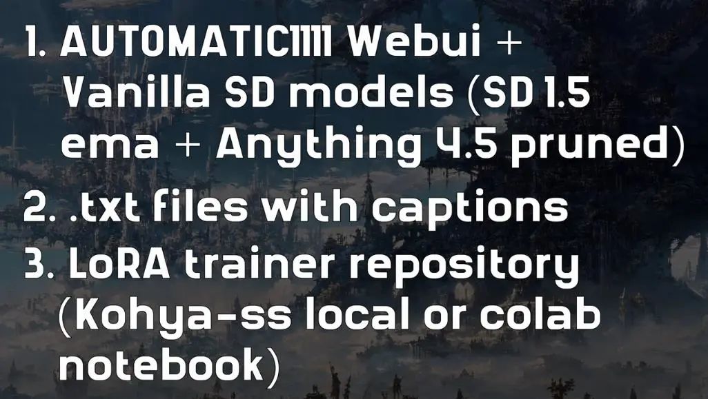
Next, you need to prepare a text file (.txt file) with descriptions, which is a key component in training the LoRA model. I will elaborate on this later.
Finally, you need a device or notebook that can train LoRA. If you do not have a powerful GPU configuration, don’t worry; you can still keep up. In fact, I will break today’s sharing into two parts: for the first part, I will use the user-friendly Kohya sd script, here is its detailed introduction (https://github.com/kohya-ss/sd-scripts), and you can learn more through the creator’s video. I will train this model on Stable Diffusion version 1.5.
For the second part, I will use Google Colab Notebook as a LoRA trainer, where I will train the anything v4.5 pruned model using my exploratory experience.
Part One: Kohya Local GUI Training
As we mentioned earlier, we will first use the user-friendly Kohya GUI. Don’t worry; the installation process is very straightforward. After copying it to your computer, enter “.
un.ps1” in the command prompt, and it will tell you the local host link (as shown).
Before proceeding to the next step, I will try to be transparent about my hardware and equipment. My graphics card is an RTX 3090 with 24GB of memory, meaning I don’t have to worry about memory overhead and can easily train my LoRA model.
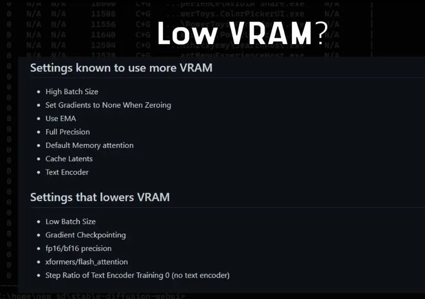
Now, if you want to learn my process but lack a powerful graphics card, that’s not a problem. You can adjust your settings to reduce the memory requirements for model training. Unfortunately, I don’t have a lower-spec GPU to test how much I can reduce the settings, but by adjusting the settings in the images (possibly turning everything off), you might be able to train on a lower-spec computer.
1.1 Dataset Preparation
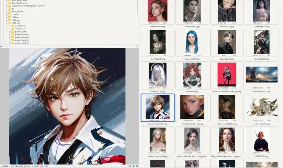
Next, I will share some tips to make dataset preparation smoother. Initially, I planned to train graphical drawings, such as the works of artist Vofan. Some of these images are from novel covers, which are illustrations he created.
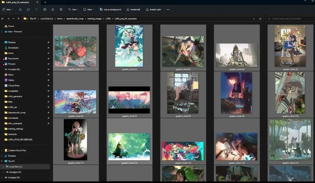
Before providing descriptions, we first need to rename these files. A useful tip is to ensure that all your files are of the same file format, such as JPG or PNG, to avoid duplicate file names during batch processing.
Here is something to avoid: in the Windows system folder, select all images and click the rename icon here. Choose a name for all images (I chose graphic_illust), press Enter, and all your images will be renamed, with the only difference being the suffix numbers changing.
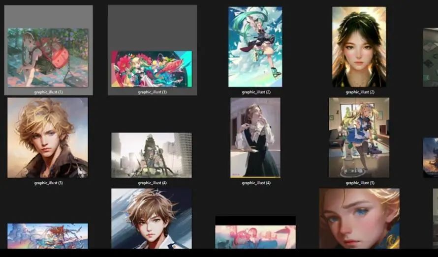 However, you can see here that there is something strange. For example, there are two files named graphic_illust (1), and we can find that almost all subsequent numbered names are duplicates. This is because my image formats include both JPG and PNG, so batch processing automatically sorted different format files, resulting in duplicate file names, which we do not want.
We need to avoid this phenomenon, but how do we do it? Here is a simple solution:
My method is to open the command prompt (cmd), navigate to the image folder, and then convert all JPGs to PNG format, or convert all PNGs to JPG, just to keep all files in your folder as the same format. So, you can type “ren *.jpg *.png” and press Enter, and all files in the folder will become PNG format.
Then, we will go back to the previous step and batch rename again (refer to previous steps), so we will not have duplicate file names.
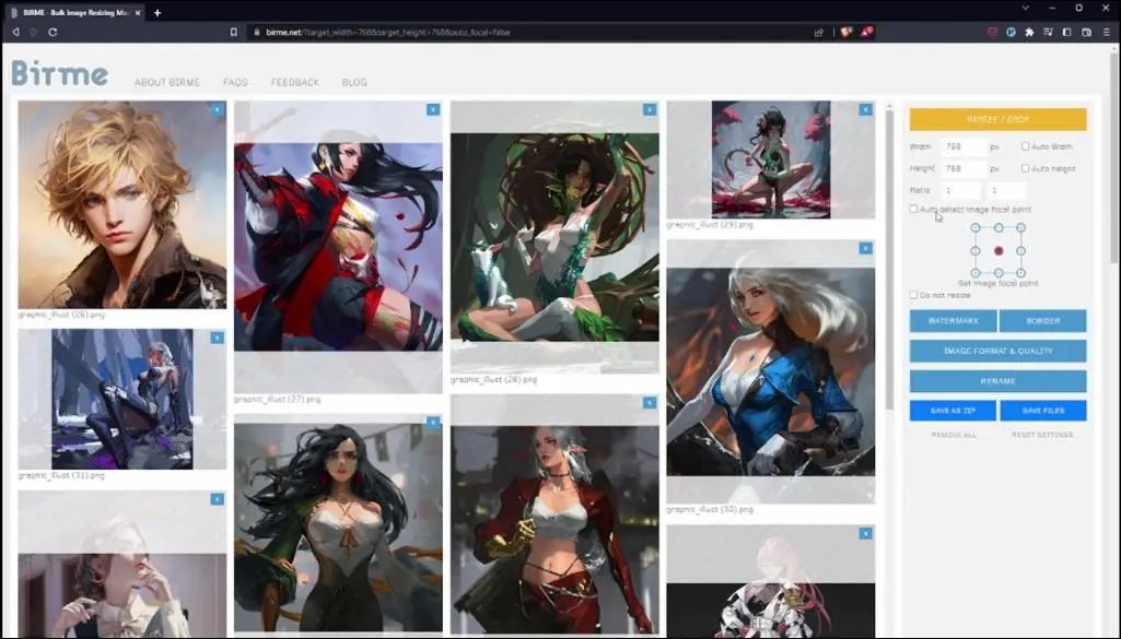
Next, place these images into an image processing tool. I used birme, and I found that my computer configuration can support training images of 768×768 size, so I cropped the images to this resolution.
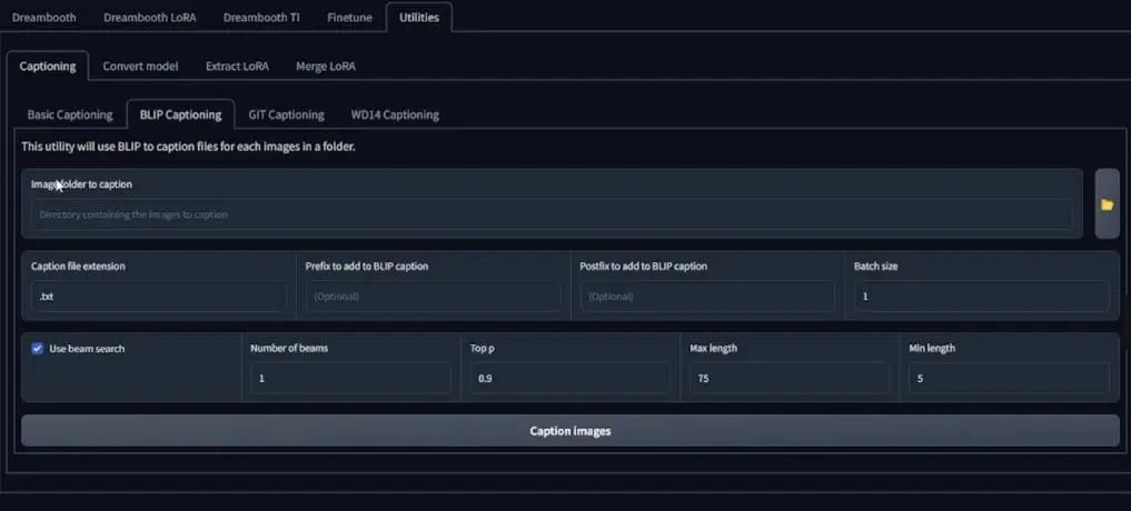
Next is to add descriptions to your images. After processing all the images, enter the GUI interface, click on the utilities tab, and select BLIP Captioning, then input your image folder (file path) into the specified location.
If you want to train a specific style, you can add a prefix here, such as entering “VOFANstyle”. However, I am not just using it to train the style of this artist, so I choose to leave it blank. Here is the configuration I selected:
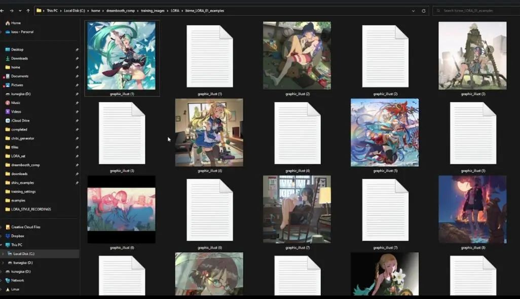
After the description processing is complete, return to the folder, and you will see that each image now has a corresponding txt description document:
The tool I use to edit descriptions is Visual Studio Code. You can see this interface; open an image file, then click the icon in the upper right corner to open the TXT file in the second window. Now, the question is, why do we add descriptions? If we want to train a character, then all images’ descriptions should refer to the same character so that it can be recognized.
So here we can replace a girl (a girl) with Hatsune Miku, but since we are not training a character, we do not need to replace it.
We want to train a style, so we will describe everything except the image style, so we will not use terms like “an illustration of” or “a photo of”. Essentially, we want to describe everything we want to change, which may be a bit difficult to understand at first, but I will try to explain it as intuitively as possible.
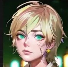
In this case, “a girl with long green hair is flying through the air” is quite accurate but not precise enough. I want to describe a teenage girl with teal eyes and long teal hair in twin tails, then remove all other descriptions and leave “flying through the air” at the end.
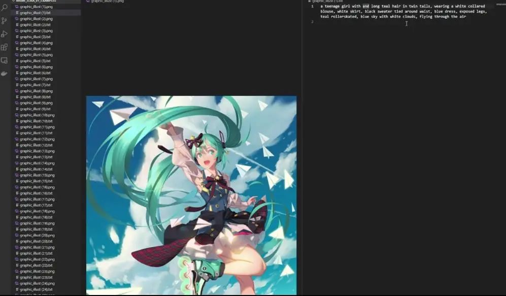
So, besides the aforementioned characteristics, what other features does she have? You can see she is wearing a white blouse, a white skirt, a black sweater tied around her waist, a blue dress, with her legs exposed, and a pair of teal roller skates. Then you can also see the blue sky and white clouds.
Complete description: a teenage girl with teal eyes and long teal hair in twin tails, wearing a white colored blouse, white skirt, black sweater tied around waist, blue dress, exposed legs, teal rollerskated, blue sky with white clouds, flying through the air
So, why do I describe so specifically here? If I don’t describe it here, it means I want LoRA to learn these things. If I don’t describe blue-green eyes, then all characters generated will have blue-green eyes. So, it is essential to describe everything that can be changed.
Here is the second image description I want to modify. You can see that the description is incorrect (a woman sitting at a table with a book and a cigarette). It is clear that something is missing, so we change it to:
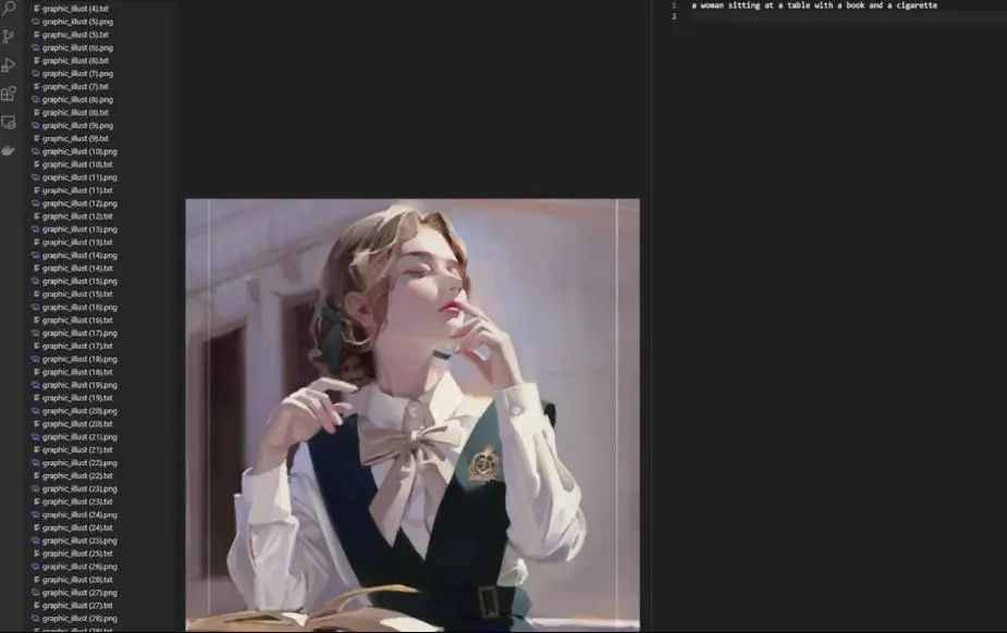
“a young woman with medium length hair, closed eyes, wearing a white colored blouse, green dress, school uniform, green hair ribbon, desaturated light brown ribbon, looking up to the right side, book in the foreground, blurry building in the background”
I think this is sufficient to describe the content in the image. Of course, this step is very time-consuming because you need to check a lot of text. If you want to obtain a good dataset, you need to handle these descriptions appropriately. So, I need to start doing these things and then start training.
1.2 Kohya_ss Settings
Now I am at the Kohya SD script deployment interface in the GUI, clicking on the Dreambooth LoRA tab, which is what we will use.
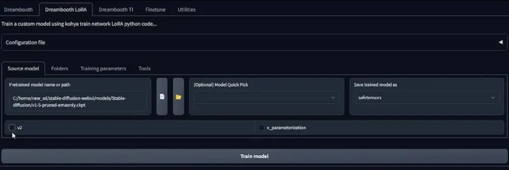
As mentioned earlier, I want to use the Stable Diffusion 1.5 version model, so click on the book icon in the image and wait for it to load the model path, and keep the two checkboxes below empty.
The next step is the tools tab. The Kohya folder is somewhat unique and must follow certain traditions. The settings in the image are what I have already set:
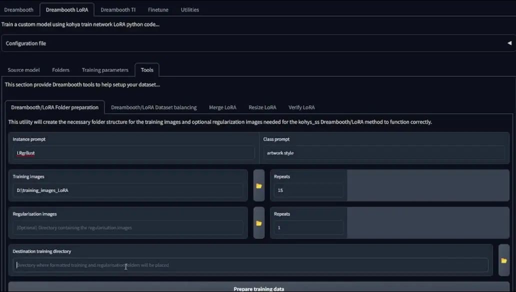
Click the Prepare Dataset button below.
Then, click the Copy Info to Folders Tab button; this is very useful.
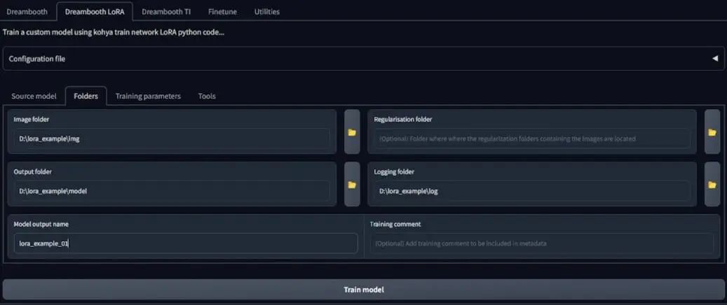
Then we come to the Folders tab. We do not need to manually enter the folder path; it has already been set in the previous step. For the model output name, I set it as lora_example_01.
Next is the training parameter settings. Open Training Parameters and see the default settings. However, since my dataset trained 157 images, these default settings may not perform well. After multiple attempts, I found that using a modified settings configuration file works much better, so I loaded them into the training parameters.
In normal LoRA model training, you might not use as many images as I do, so you can increase the training frequency since I’m using very low numbers. Then we will discuss other settings in detail.
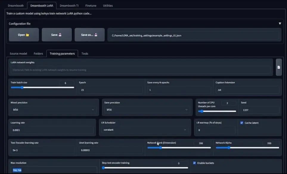
For training batch size, if your GPU memory is less than 8GB, I suggest setting it to 2 or even 1, which represents the number of parallel computations you can run simultaneously. Next is the number of epochs, which represents how many times you propagate through a dataset. You can adjust this number, but I strongly recommend at least greater than 1 because it will become your snapshot file (snapshot file) or the saved LoRA file.
In the end, I should have 15 LoRA files, one for each epoch. You need these files because they represent different time points, and you can use them to check if your results are overfitting.
Next is the precision. If you can use the bf16 precision model, be sure to use it. If there is an error during training, use fb16. For the LR Scheduler settings, just choose constant. The training frequency is default, and if your text encoder or unet learning frequency is blank, it will use the default value.
Then there are the network rank and network alpha settings. Generally, you should keep the same or similar values as mine. For high-resolution images like 768×768 pixels, using a higher network rank is a good idea. For stylized training of non-anime models, setting it to 200 or better would be preferable.
Based on my personal experience, when the value is around 256, you will start to get poor results, so I suggest not setting it that high. Alternatively, if you want such high settings, you need to lower the unet learning rate further.
Then there are advanced settings, and you can see my settings. You can match my settings because the Stable Diffusion 1.5 model is trained based on CLIP SKIP1, so keep its value at 1. For anime models or other V3 versions, set clip skip to 2.
I also enabled shuffle captions. If you find that LoRA training has some color issues, you can enable the color augmentation feature, but it will subsequently disable cache latent on this page. So, if color becomes a significant issue, you can attempt to enable this feature.
In summary, these are the settings I used, and now we can start training the model. But before that, I need to mention a small detail, which is the step count, which will appear in the console output. If your training batch size is greater than 1, the total training steps will actually differ significantly because it is the product of the number of images, repetitions, and epochs. I used 157 images, so my training steps are 35325.
However, my training batch size is 6, so I need to divide the total steps by 6. As I mentioned before, this is the number of parallel computations you run simultaneously, so the result is about 5888 steps. When I actually train, the result presented is 5888 steps, not the total steps of 35325.
If everything is ready, you can press the train button to start training.
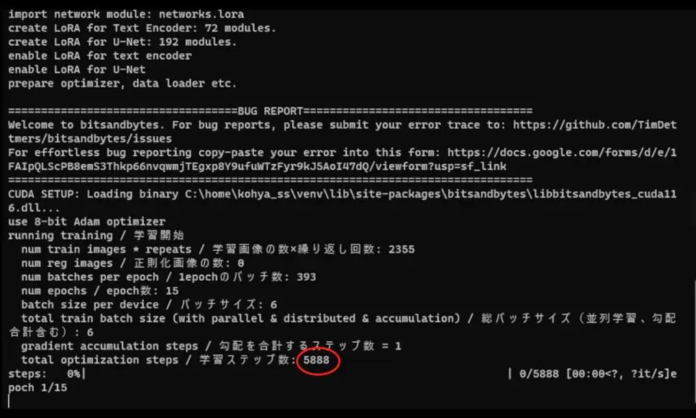
If you check the power shell, you can see the maximum training steps are 5888, followed by loading my checkpoint, and then possibly cache latents.
Now it will calculate the steps. For me, the total training time is about 12 to 15 hours, but this is for 15 epochs, 157 images, and a high resolution with a network rank of 200. So, this is not a standard training time; if the training numbers are reasonable, the training time for LoRA is between 30 minutes to 2 hours.
1.4 Analyzing Results
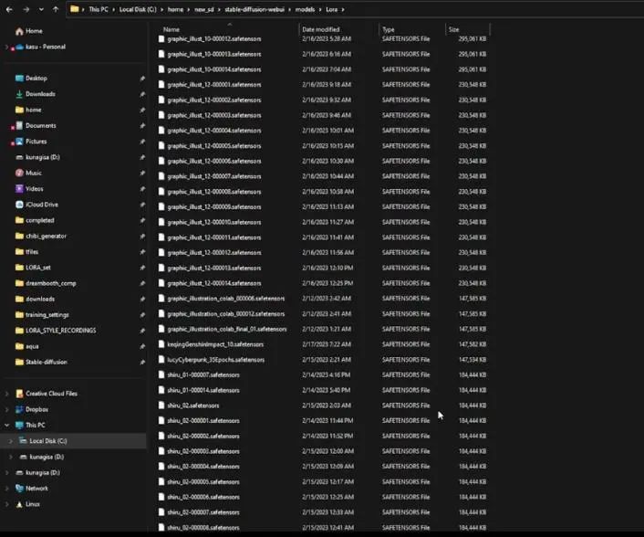
If your training did not encounter any errors, then congratulations. Enter the folder you created, and then open the model folder. You should see as many files as the number of epochs, so I have 15 files here. Select all and copy them into the Stable Diffusion LoRA folder (stable-diffusion-webui/models/lora), ensuring all files are here; otherwise, you cannot proceed to the next step.
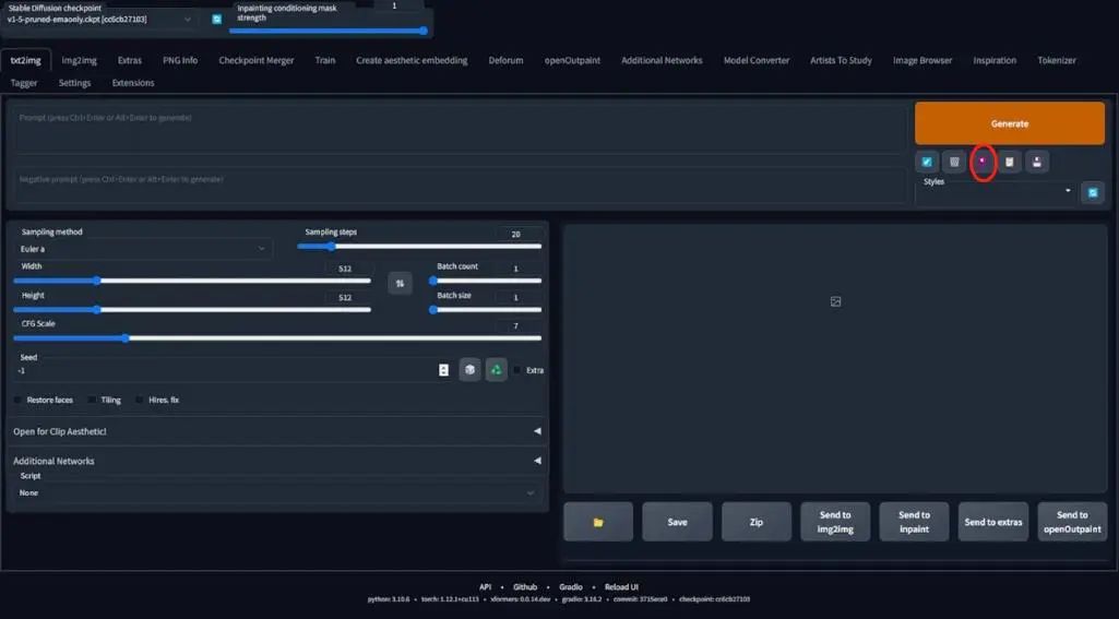
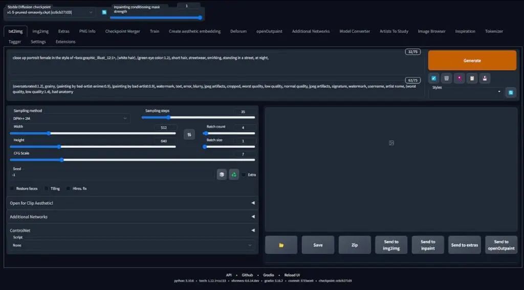
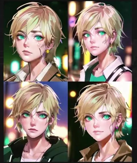
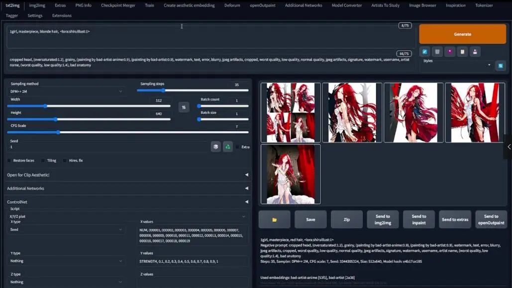
Next is to analyze our LoRA model. My method is to choose a very standard and simple prompt and negative prompt to activate and use your LoRA model. Click the red button here, go to the LoRA tab, and search for your LoRA name; mine is graphic_illust_12.
Select one, and LoRA will appear in this form. Then, the way I write prompts using LoRA is as follows:
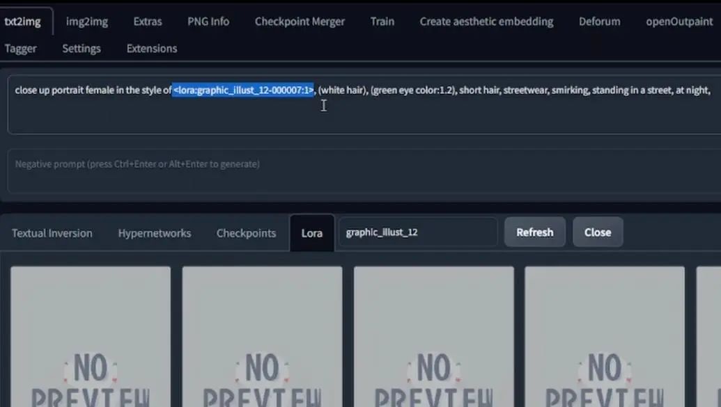
This is how I tell Stable Diffusion to load LoRA style learning information, then paste the negative prompt, and set the sampling method to the one I usually use.
Next, I open XYZ selection under the script options. Remember that the number of epochs is saved in the format of the LoRA name, so here it is illust_12, followed by five zeros and an integer. The LoRA weight or strength is after the colon. I want a grid that not only displays variants of the epoch model but also changes the LoRA weight.
To do this, I will first select Prompt S/R for the X type, representing search and replace. Here, I want to replace the model number, so I will change 000007 to variant num, and then in the X value, I will write NUM, 000001, 000002…..0000014.
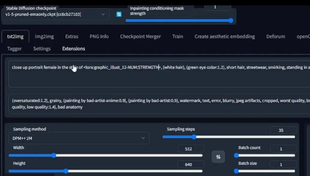
If you understand this logic, then the following will be straightforward. For example, for the Y type, select Prompt S/R, and then input STRENGTH, 0.1, 0.2……0.9, 1. And change 1 to strength, so that after entering the prompt, I will at least get a 14×10 or 10×14 grid of display variants. Don’t forget to select the model as the one you trained; here I have selected 1.5 pruned-emaonly, so choose different things based on your actual needs.
Next, I input the prompt, and it looks like the grid has been generated. Clicking on it yields the following effect:
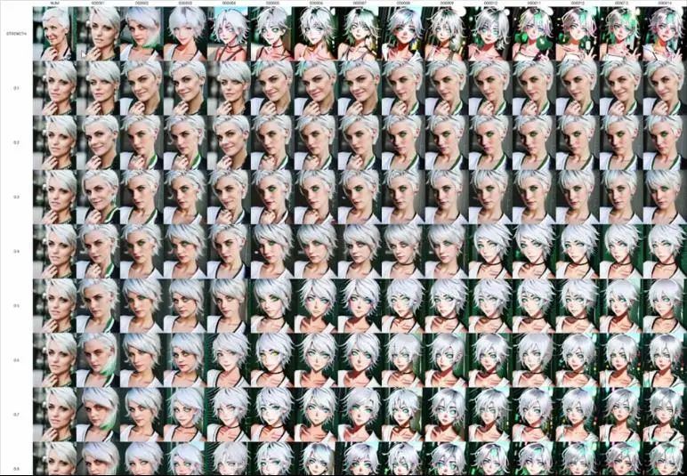
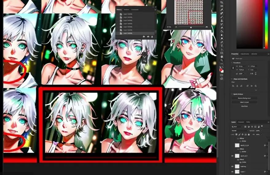
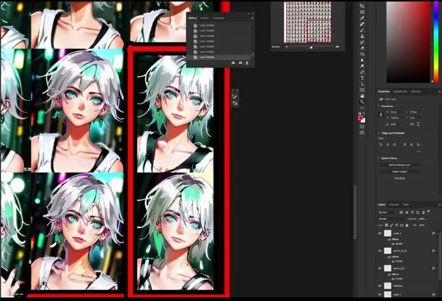
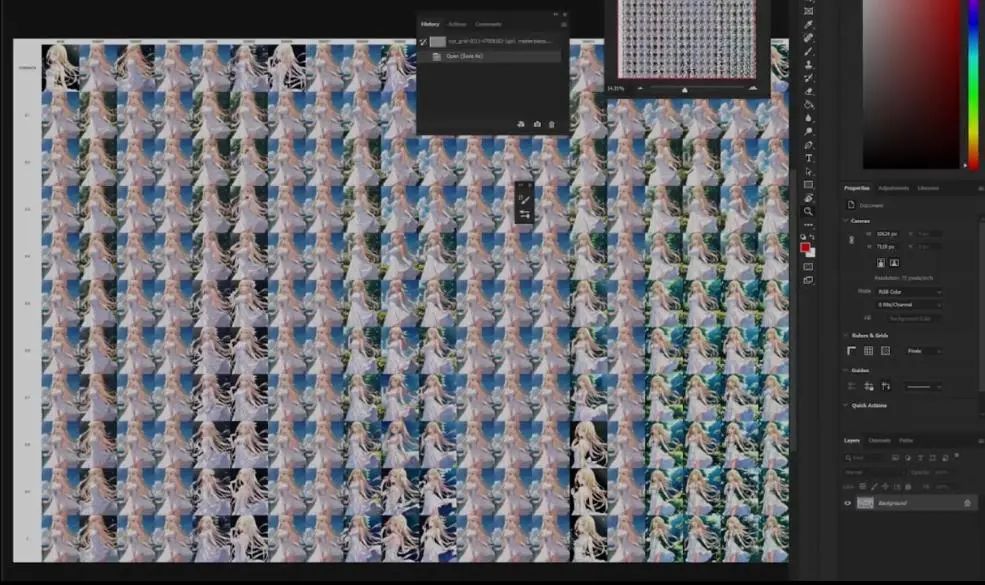
I think it is best to go into the output result folder and put it into Photoshop for better observation. The images are too small to tell if there is overfitting.
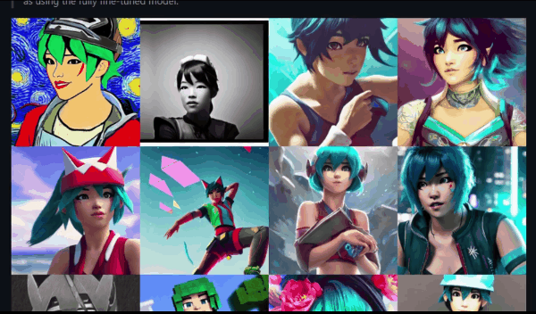
This is the view in Photoshop, where the horizontal axis is X and the vertical axis is Y. At this point, we can decide which epoch to further test. Some suggest that at a LoRA strength of 1, there should be no overfitting. Fortunately or unfortunately, after many attempts, we did not get particularly poor results.
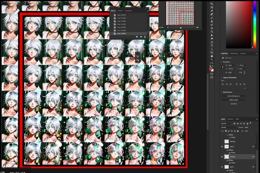
Next, focus on the lower right corner of the grid, where we can see the results of higher LoRA strength and epochs. More epochs mean longer training processing time. Personally, I want to start analyzing epoch 7, as the image shapes are clearer, and the strength is 1.
If you know games, the final world reminds me of this style:
Even though the data did not have such a style.
Here, there are even hatching marks, which is a pleasant surprise.
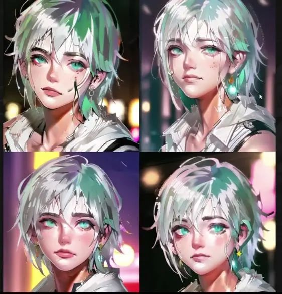
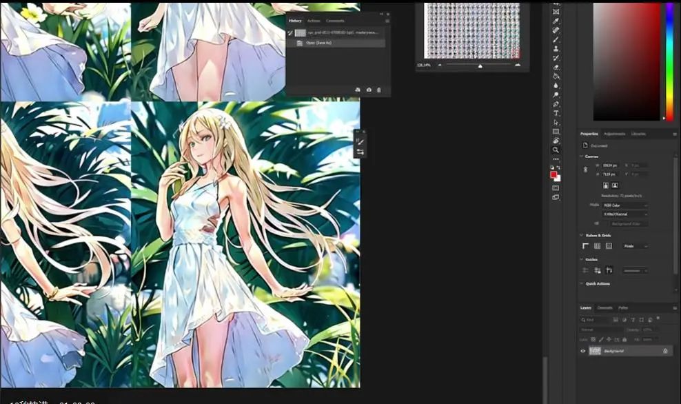
Then, if we continue to increase the number of epochs, you will see some confusing things. For example, the mascara or eyeshadow in epochs 8 and 9, but they disappear in epoch 10. At a strength of 1, from epochs 10 to 14, we start to get very good illustration effects, actually achieving what the dataset wants it to do, or what I want the LoRA model to achieve.
However, in the second to last epoch, we found some artifacts, so epochs 13 and 14 got a bit out of control. If we analyze the results roughly, we might abandon the last few epochs due to overfitting.
If we look closely, we will find that epochs 14 with strengths of 0.8 and 0.9 perform very well. So personally, based on experimental results, I will continue and test the final 15 epochs in the webui to see if it truly overfits or if it’s because I used a poor seed number during generation. So we start to try:
1.5 Determining the Final LoRA Model
Here we enter the stable diffusion webui interface. I want to test the final epoch, and there will be no numbers attached, so we will test with a random seed and strength set to 1.
These are our results, and personally, I like them. If you don’t achieve the desired clarity, you can lower the LoRA strength to 0.9 or lower.
We keep the seed number and lower the strength to 0.9, and you can see that the artifacts disappear. Of course, these areas can always be improved through local repainting, so I’m not too worried about the text-to-image part.
So, why don’t we try other options? For example, changing the white hair in the prompt to golden hair means our LoRA model is not restricted. If we cannot change the output result through variations in the prompt, it indicates that our LoRA model has overfitted, which is another thing we should notice.
If the result is golden hair, like in the image, then we can continue. This is how to test the LoRA character.
But what if the result is something that the LoRA model has not been trained on? This is also the purpose of our style training, so I prepared some prompts for testing.
1.6 Applying LoRA Style
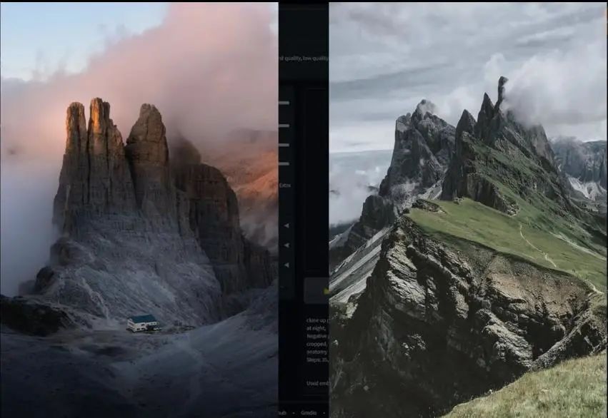
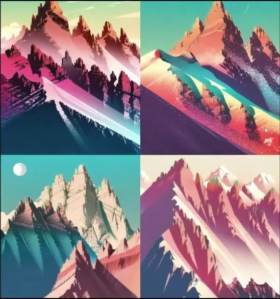
Here we remove the character-related content from the prompt, set the strength back to 1, and change the seed to random (-1). We can first test the generation of an outdoor scene, such as the famous Dolomites in northern Italy, and see if it can generate associated graphics.

You can see that the result is quite good; its shape is consistent with the Dolomites, but in a different style.
Then, is it feasible to change to an indoor scene? For example, a library, we can get illustration-style images.
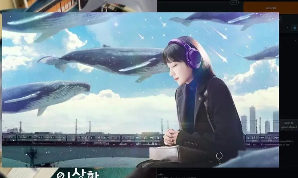
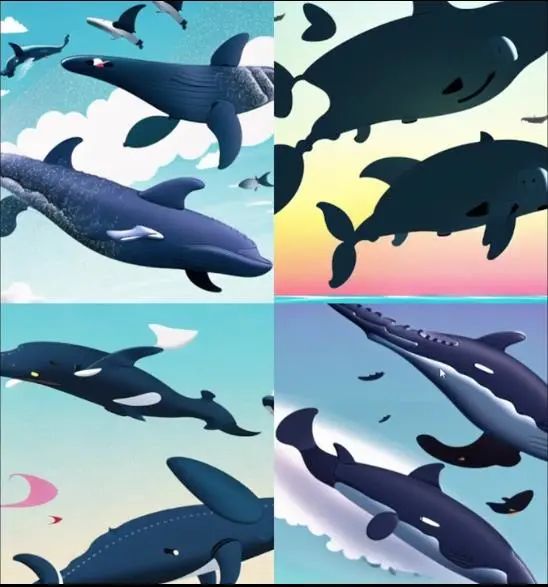
Then we can test something very random, such as the Korean drama “Extraordinary Attorney Woo”; she likes flying whales, so we can modify the prompt to flying whales and see what results we get:
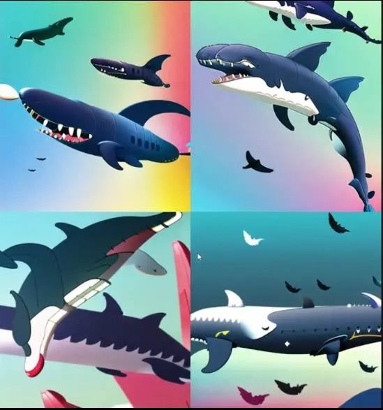
These results are cool; I personally like them. If you find them too intense, you can lower the strength, but even at a strength of 1, there are no artifacts. We can modify it to 0.8:
From my analysis, no matter what prompt you input, the LoRA model will not exhibit overfitting. Of course, it may also be that I have not found the right testing method to discover overfitting. However, I think this is a good attempt.
So, next, I will start LoRA training in anime style, which I believe many people will be interested in.
Part Two: Training Kohya LoRA Model with Google Colab
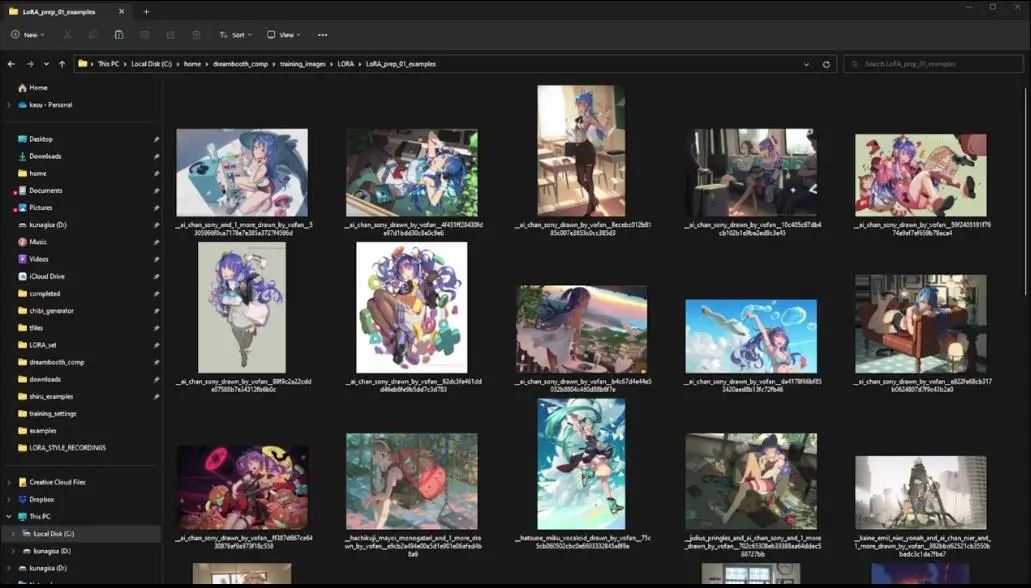
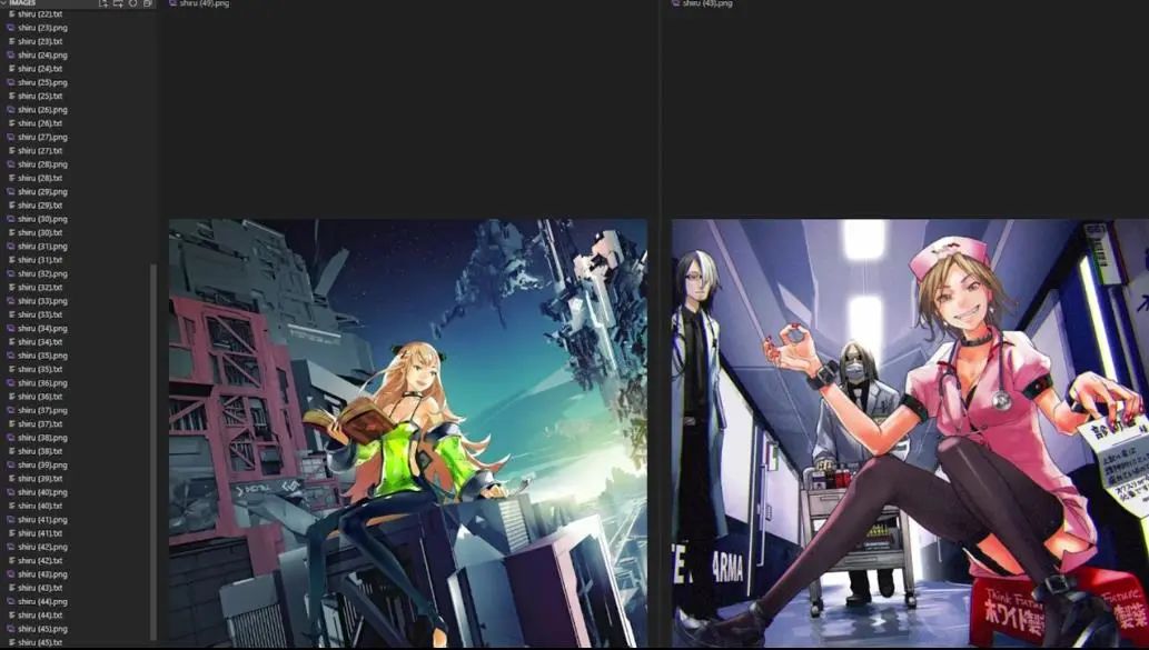
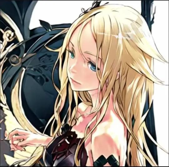
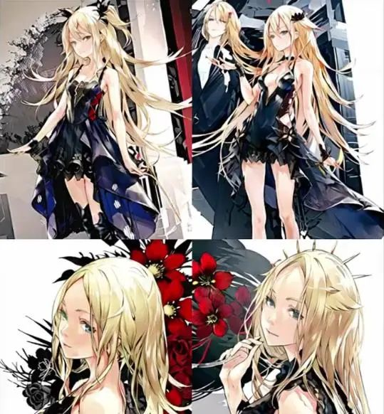
Before starting to train LoRA, we need to start with the dataset as usual. Here I choose the works of Japanese illustrator redjuice, who is also well-known by many under the name shiru. Shiru means soup, and here I choose images of 768×768 pixels. If you are not familiar with how I prepared the dataset, please refer to the first part.
Here you can see that all images have the same name, with the only difference being the suffix numbers, and they are all in PNG format.
2.1 Dataset Preparation
Since this assumes you will not use the Kohya local installation but will use Google Colab, I have changed the process of adding descriptions to use the tagger web extension in AUTOMATIC1111.
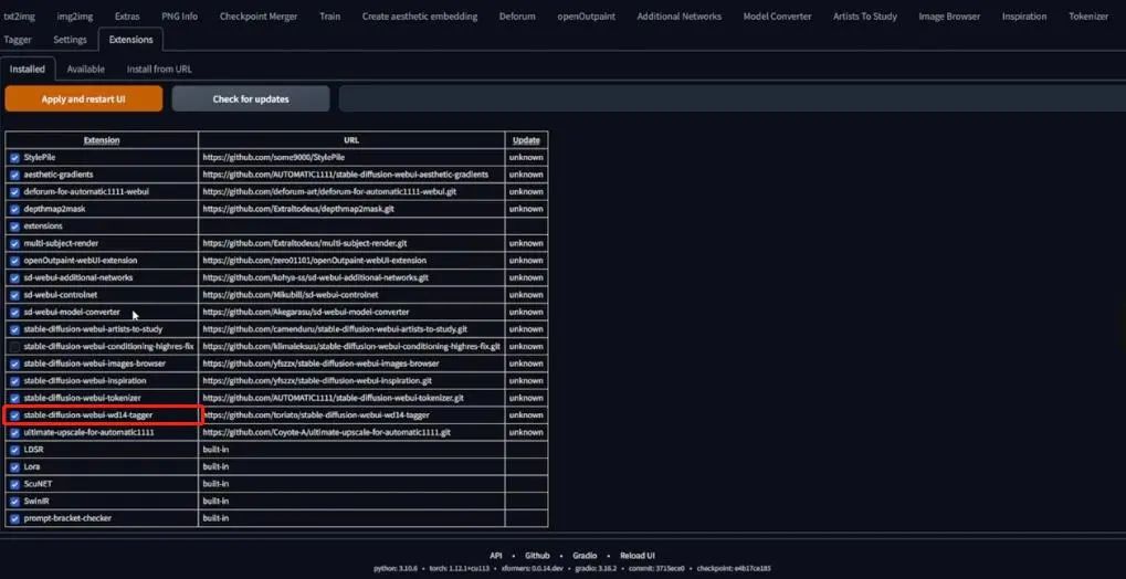
So, click on extensions, and you can see that I have already installed the tagger. Then click on the Tagger tab, and you will see the following interface:
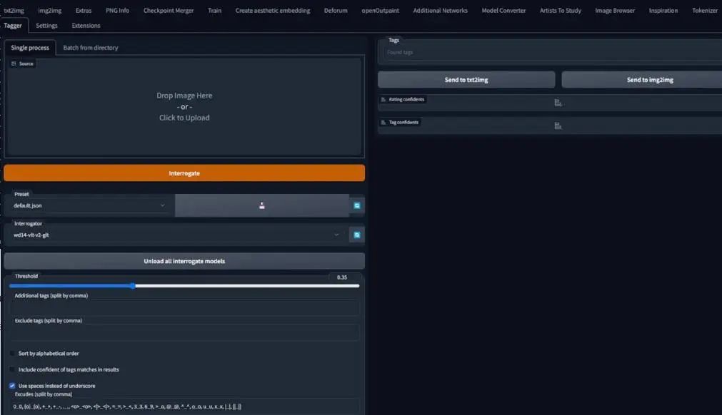
The description process here is different from the first part (blip captioning). Since this time we will use the clip skip 2 model for training, usually for anime styles, here is the v4.5 Pruned model. Be sure to ensure the use of Danbooru style tags, and you will soon know what I mean.
Click the “Batch from Directory” tab, and input the correct path in the input directory. If you want to add a tag before other tags, such as redjuicestyle, I usually do not use tokens to reference styles, so I will leave it blank. Therefore, I do not know the best way here. If you understand the first part, you will know that such choices are also very good for LoRA.
If everything meets your needs, click the interrogate button and then check the console:
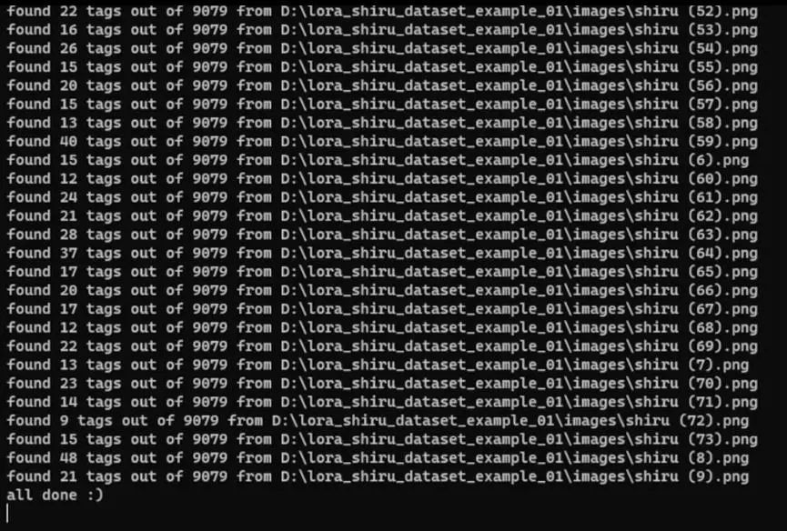
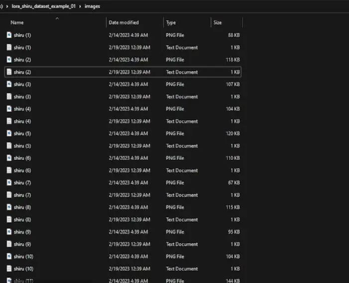
It is loading these files. Once completed, we jump to the dataset folder to see if there are description files.
2.2 Improving Descriptions
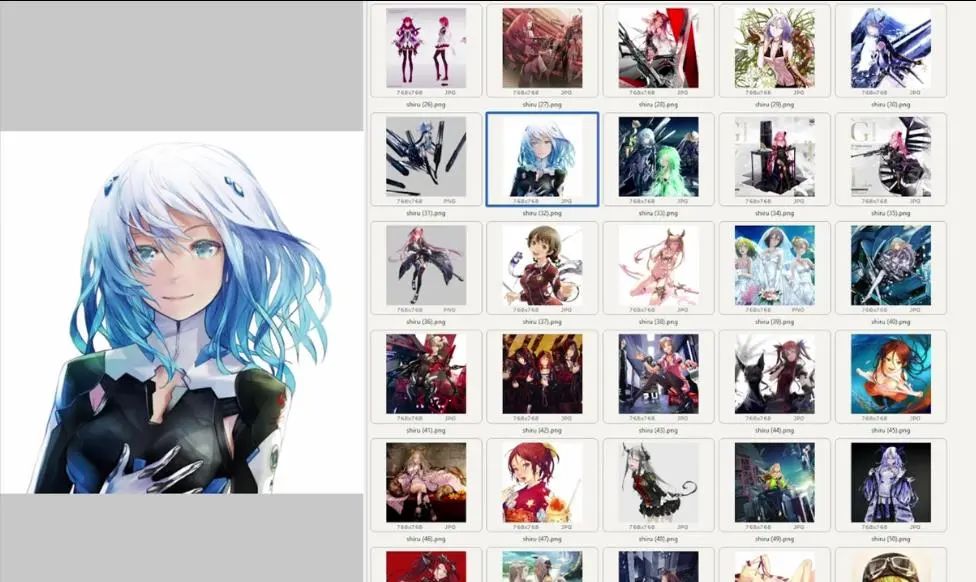
We can see that each corresponding image now has a description file. However, we are not finished yet; we still need to open the VS Code software again for editing.
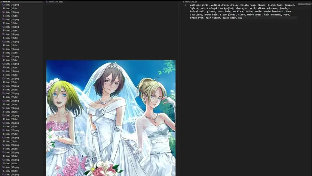
This is the VS Code interface. On the left is the images in my dataset, and on the right is their description text. At first glance, we can see that many of them are correct. For example, wedding dresses, gloves, elbow gloves, coronets, white dresses, etc., are all present in the image.
I do not want to modify every detail, but there are some things that need to be changed here, such as the character descriptions that reference names, like Mikasa Ackerman, Annie Leonhardt, Ymir (which do not exist in the image), and Christa Renz. These names are problematic for us. As mentioned in the first part, we want to describe everything we want to change. If we leave the names, they will act as markers and affect the final style of LoRA.
We want LoRA to compromise only on a single concept for each image, so we should remove all character names and then check all description files to remove the names.
2.3 Kohya Colab Notebook
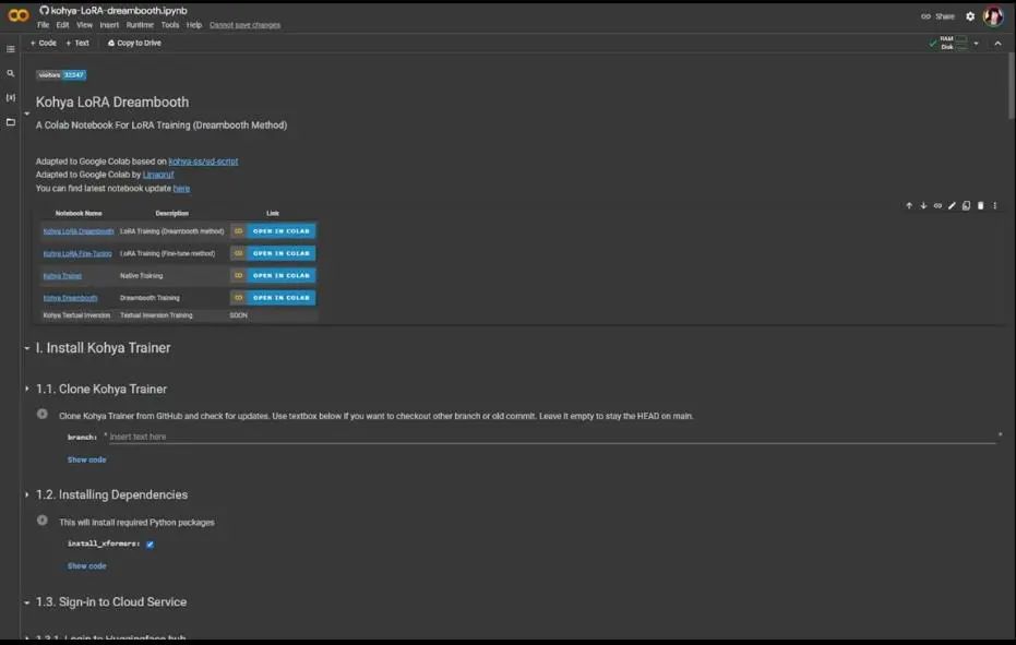
Now that our dataset has been appropriately described, we proceed to the Google Colab Notebook, as shown. Its purpose is very intuitive, but I will introduce it one by one.
The first part is Clone Kohya Trainer. You only need to press the play button, and it will prompt you that Kohya has not been certified by Google; just choose to run it, and once completed, there will be a green checkmark.
Next is to install dependencies. Click the corresponding play button again, and it will start processing and installing Python packages, which will take a while, so you need to wait for everything to complete.
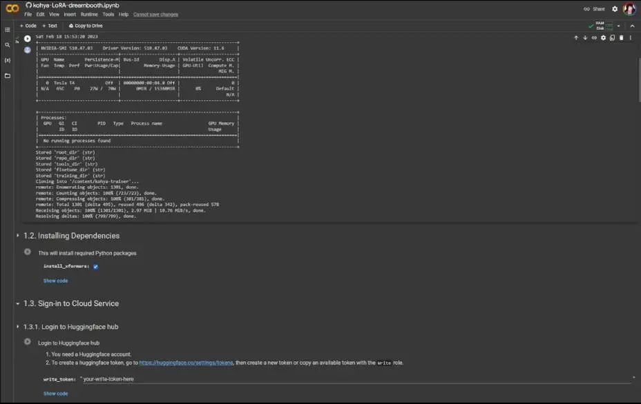
Then, in 1.3.1, log into the Huggingface community, make sure you have a Huggingface account and a token with write permissions. I will paste my token here and click the play button.
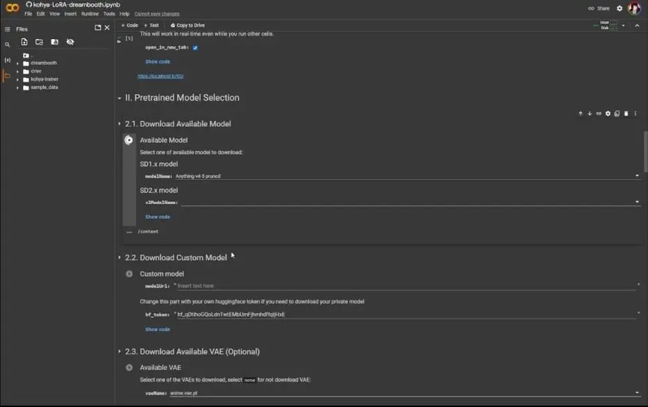
The next step is to Mount Drive. Click play to connect to Google Drive, and once completed, click the folder icon on the left to see the drive folder.
Then, open a special file browser for Colab by clicking the play button and waiting for completion.
The second part is to download the model you want to use. I am using Anything v4.5 pruned. After selecting, click the play button, and it will begin downloading and syncing from Huggingface.
You can skip 2.2 since we won’t use a custom model, so we go directly to 2.3, downloading the available VAE. We are using an anime style, so the option is anime.vae.pt. Just click the play button.
The third part is data acquisition. Define your training data location and set the training repetitions to 10; you can change the others as they don’t have much impact. After clicking the play button, it will create a folder on the left, located within the Dreambooth folder.
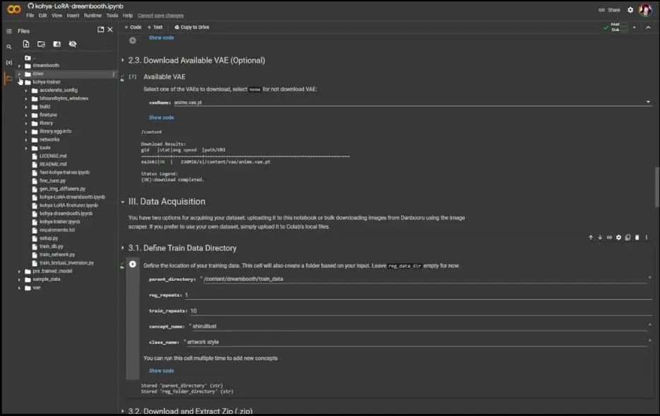
Then, upload the dataset. The rest of the third and fourth parts can be skipped since we prepared the dataset locally.
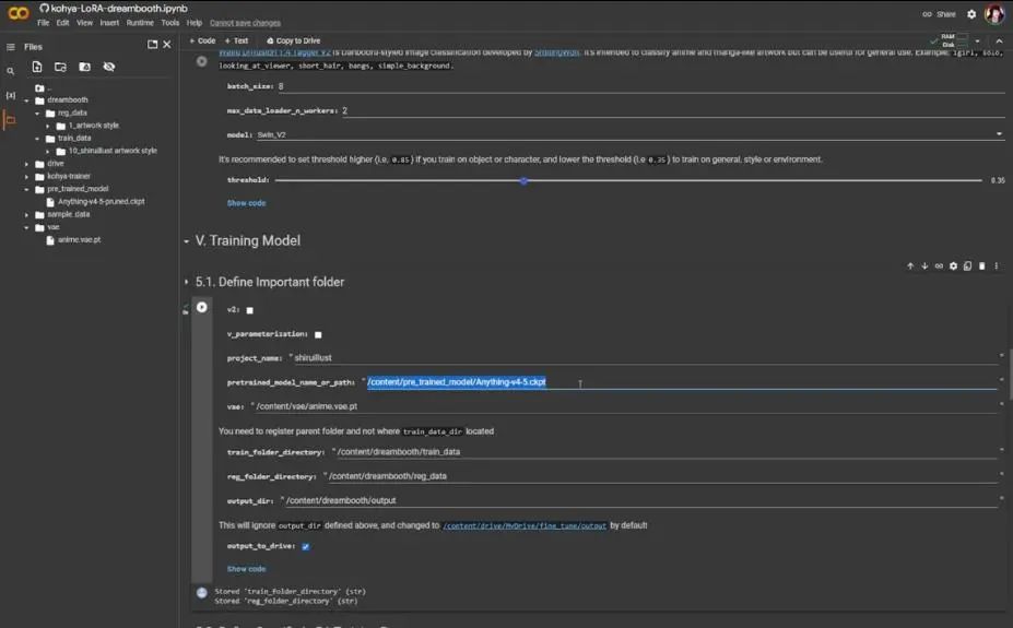
Next, define the essential folders, which is the fifth part. Set the project name to “shiruillust”, change the pre-trained model path to Anything -v4-5, and change the suffix Safetensors to ckpt (i.e., checkpoint).
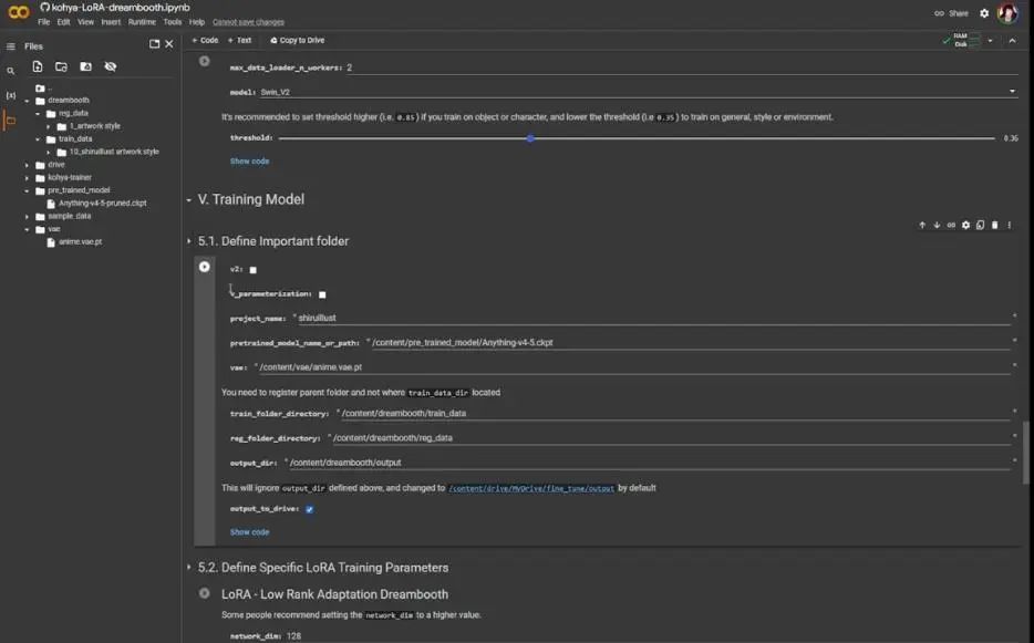
For VAE, we already have one on the left, click to copy the path and paste it into the corresponding position. The other settings look okay, but for the output directory, I want to change it to the local hard drive, so check output to hard drive. Then click the play button to start defining my folders.
Since we skipped data uploading, you need to go to the local dataset folder, select all, and then drag them to the training data folder on the left.
This is my Kohya training setup. I set the epochs to 20, changed the learning rate to 0.0001, and selected a network rank of 160. So, back to Colab, set the network dim in section 5.2 to 160 and the learning rate to 1e-4, with the other settings as shown.
Then click the play button.
Now, start LoRA Dreambooth. I choose fb16, but I don’t think the Colab GPU can handle it, so keep it at fp16. You can set the resolution to 768, as I did in local training, but this may cause the program to crash due to insufficient memory, so keep the resolution as low as possible, usually set to 512; the settings here are 640.
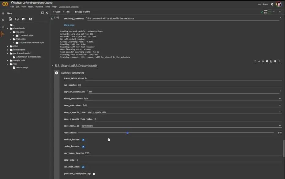
Set the number of epochs to 20, set save_n_epochs_type to save_every_n_epochs, and set the save epoch type value to 1, so it will save from 0.1, 0.2 all the way to 1 like in the first part.
The other settings look okay, and you can check the code to see if there are any numerical errors. If everything is fine, you can click the play button.
Here we find an error, which is a good thing because I made a mistake. You can see that my local path was incorrect, so I went back to the pre-trained model path. I did not write “pruned” in the path, so it’s best to copy the path directly and paste it, then run 5.2 again, and then run 5.3.
This will take some time, about an hour and a half, so just wait for it to complete.
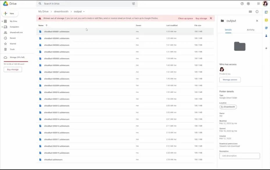
If you want to know where your files are, go into Google Drive, and you will see the Dreambooth folder under My Drive. Everything should be in the output folder here. Open it, and you can see all the epoch results. The final result is a file without numbers.
You can select all, right-click, and choose download. They will be packaged into a Zip file, which you can unzip and copy into the LoRA model folder under Stable Diffusion, then open the webui.
2.4 Analyzing LoRA Model
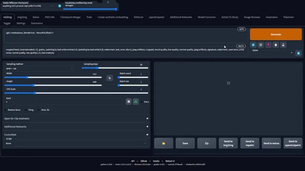
Now we enter the webui, which has loaded LoRA. My name is shiruillust, and I will select the last file without numbers, run it, and see if it works.
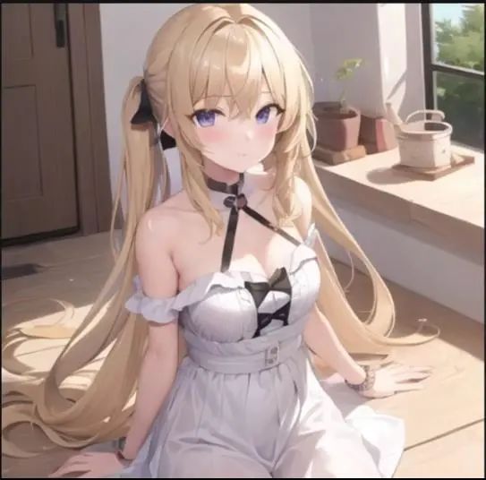
First, delete LoRA, generate an image as a seed, then paste the LoRA model, paste the image seed code into the seed, and click generate. It should give me a stylized result:
You can see that the resulting image indeed has the redjuice style.
We change the batch size to 4, set the seed to random, and then check the results:
The four images look a bit rough, but they still seem feasible. So, next, we repeat the steps from the first part to create an image grid.
But before that, let’s see if we can change some content in the images, such as changing the blonde hair to red hair. If the resulting image does not change, then it indicates that our model has issues:
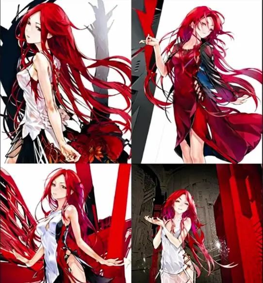
You can see that it can change the character’s hair color, and some images even change the color of the dress to red. To achieve precise control, we just need to write the prompts more specifically later.
Go back to the script options, copy and paste the XYZ values used before into the corresponding positions. However, here the epoch is 20, so we need to increase NUM to 000019, keeping the rest unchanged.
Then, change the batch size to 1, change the numbers in LoRA to num and strength, ensure to use Prompt S/R, and then click generate.
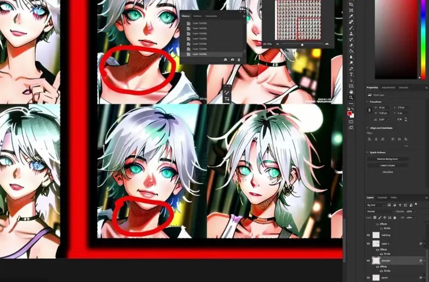
We open the resulting image in Photoshop and only look at the results of the last few epochs. By about epoch 9, there is a hint of the redjuice style, and by epoch 14, we can see significant changes. I will only select the last epoch, as it should provide the best results.
So, I go back to Stable Diffusion and perform some generation tests with the final epoch.
2.5 Validating the Final LoRA Model
Indeed, there is the redjuice style.
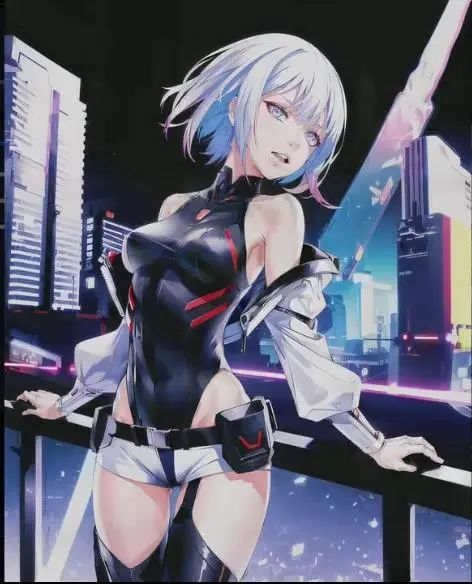
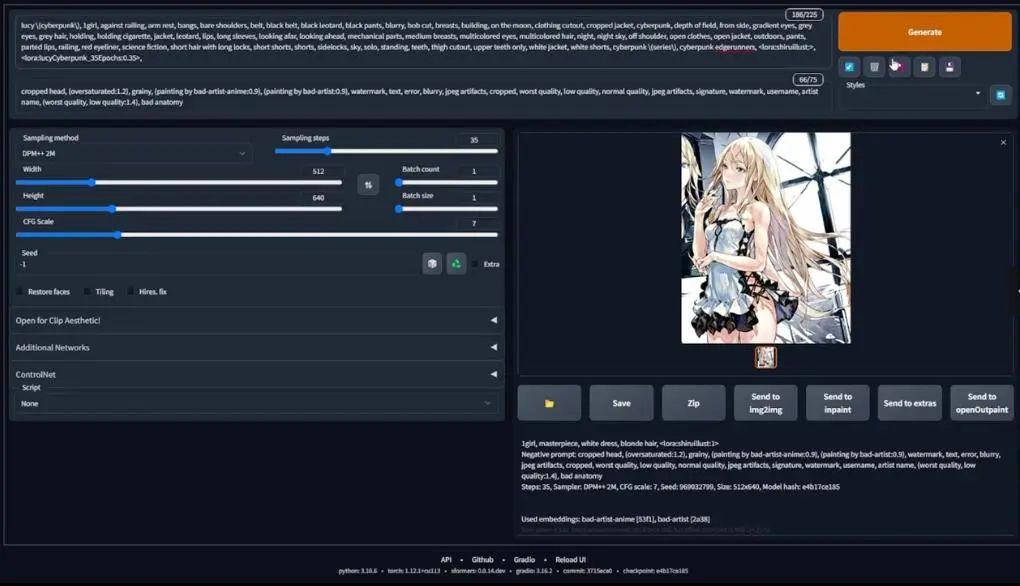
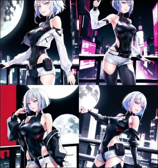
If you remember from the beginning, you will find a cyberpunk character named Lucy in the redjuice style, so we will test whether the model can generate corresponding results by combining LoRA models.
2.6 Combining LoRA Models
Here we paste the prompt. The original code is for the local training version, but I will change it to the Colab version to see if it works.
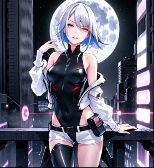
Redjuice style Lucy.
Increase the batch size and see if it still works:
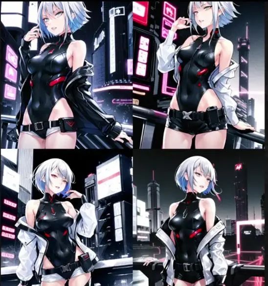
The generated results are satisfying.
However, you could do more repetitions or more epochs during the training phase, as too few steps may seem a bit insufficient.
Then generate with the locally trained LoRA model, and you can see that the results are better:
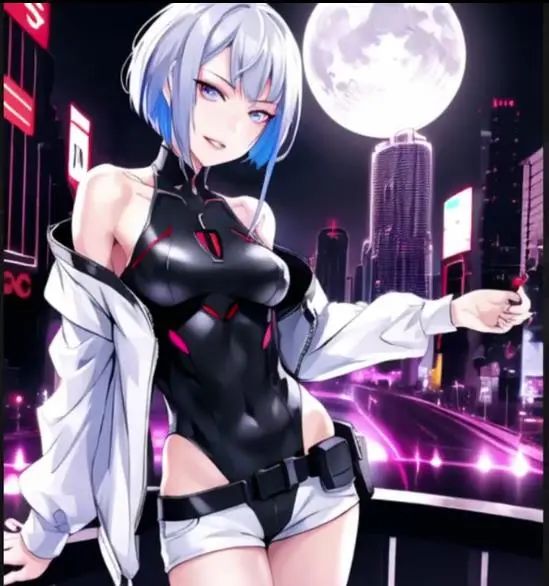
But this may also be because I used VAE.
It doesn’t seem to make much difference.
Next, I will try another style for LoRA model training in Colab. This time we will test a character named Aqua from “Kingdom Hearts”:
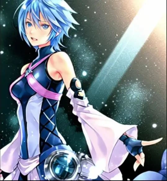
It looks like Aqua.
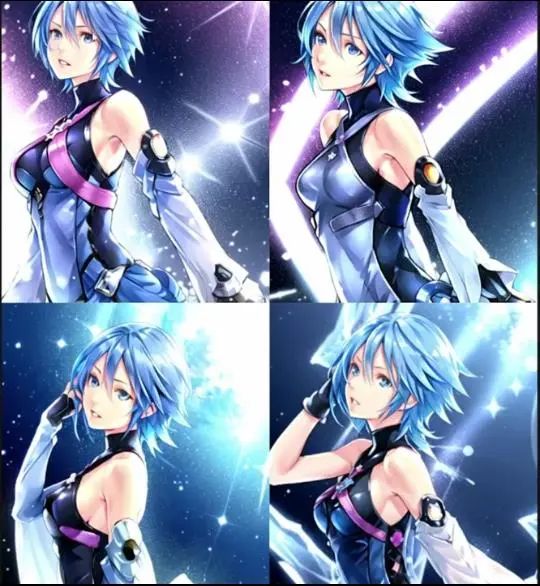
Setting the batch size to 4, we can see that the style is consistent and does indeed look like it was drawn by redjuice. If you want to maintain unsaturated colors, you need to remove the VAE. Let’s try:
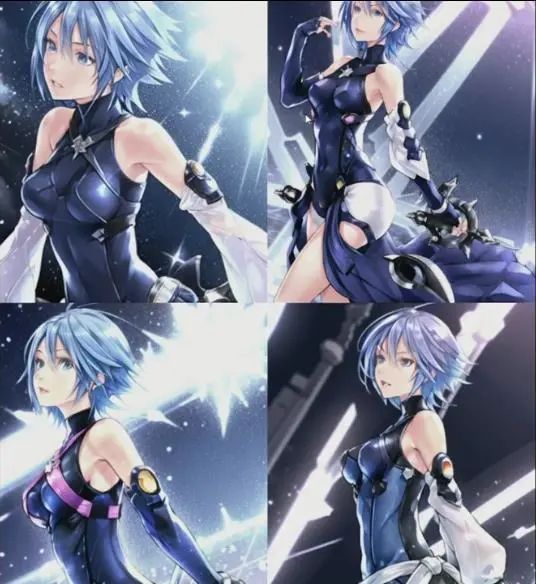
Some images do not have the pink ribbon, so we need to lower the character LoRA style or character strength, but the overall result is now complete.
Let’s test Lucy without VAE:
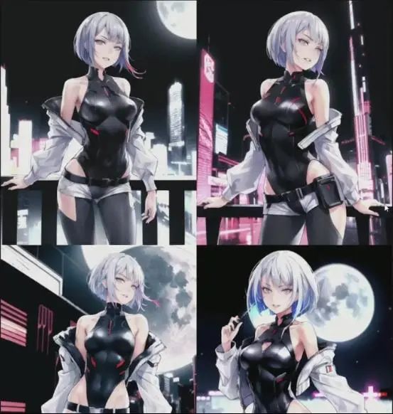
Here, the redjuice style is more evident.
All the models I trained can be found on Civitai, and I hope you can find the style training methods you need. However, I am still experimenting, and these methods have indeed brought me satisfactory results, and I hope it can help you too.
····· End ·····
GameLook Daily Game Industry Report
Global Vision / In-depth Content
Report / Communication / Cooperation: Please add the editor’s WeChat igamelook
Advertising: Please add QQ: 1772295880
Long press the image below, “Scan the QR code” to subscribe to the WeChat public account

····· For more content, please visit www.gamelook.com.cn ·····
Copyright © GameLook® 2009-2023
If you think it’s good please click here ↓↓↓