
Click on the above “Visual Learning for Beginners“, select to add “Starred” or “Top“
Heavyweight content delivered first-hand
In the field of CV, what else can transformers do besides classification? This article will use a word recognition task dataset to explain how to use transformers to implement a simple OCR text recognition task, and experience how transformers are applied to more complex CV tasks beyond just classification. The article is divided into four parts:
1. Introduction and acquisition of the dataset
2. Data analysis and relationship construction
3. How to integrate transformers into OCR
4. Explanation of training framework code
Note: This article focuses on how to design models and training architectures to solve OCR tasks. The article contains complete practices and the code is quite long, so it is recommended to save it. Those unfamiliar with transformers can click here for a review.
The entire text recognition task mainly includes the following files:
– analysis_recognition_dataset.py (Dataset analysis script)
– ocr_by_transformer.py (OCR task training script)
– transformer.py (Transformer model file)
– train_utils.py (Training related auxiliary functions, loss, optimizer, etc.)
Among them, ocr_by_transformer.py is the main training script, which relies on train_utils.py and transformer.py to build the transformer for character recognition model training.
1. Introduction and Acquisition of the Dataset
The dataset used in this article is based on ICDAR2015 Incidental Scene Text in Task 4.3: Word Recognition, which is a well-known dataset for text recognition in natural scenes. This time, to simplify the difficulty of the experiment, we removed some images from it, so the dataset in this article is slightly different from the original dataset.
In order to better share data and manage versions, we chose to call the dataset online, storing the simplified dataset on a dedicated data sharing platform. The open-source address for the data is: https://gas.graviti.cn/dataset/datawhale/ICDAR2015 , and related issues can be discussed directly in the dataset discussion area.
This dataset contains text regions appearing in numerous natural scene images, with the training set containing 4326 images and the test set containing 1992 images. They are all cropped from the original large images based on the bounding box of the text region, and the text in the images is mostly located at the center of the images.
The images in the dataset are similar to the following style:
| word_104.png, “Optical” |
|---|
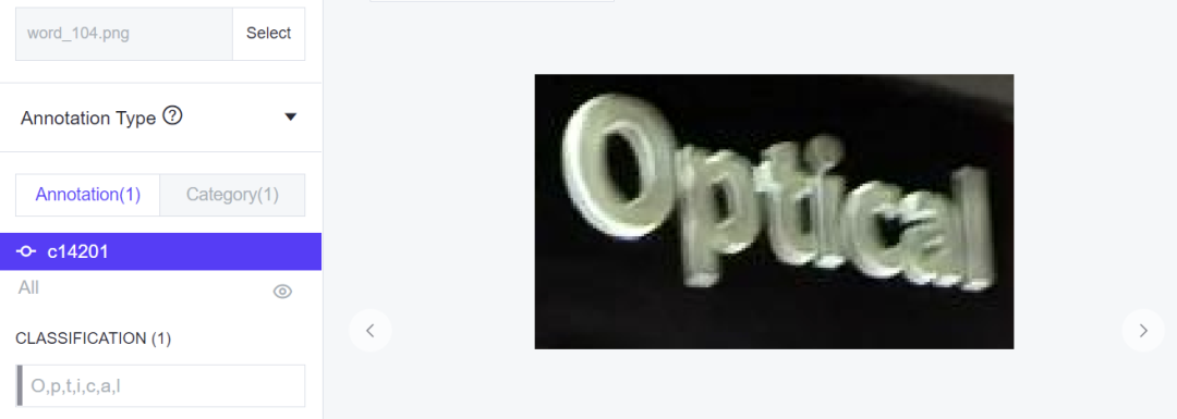 |
The data itself is displayed as images, with corresponding labels stored in CLASSIFICATION. In the subsequent code, label acquisition will directly obtain a list of all characters, which is also a storage choice made for the ease of label usability.
Below is a brief introduction to the quick use of the dataset:
-
Download and install tensorbay locally
pip3 install tensorbay
-
Open the dataset link in this article: https://gas.graviti.cn/dataset/datawhale/ICDAR2015
-
Fork the dataset to your account
-
Click the developer tool at the top of the webpage –> AccessKey –> Create a new AccessKey –> Copy this Key
from tensorbay import GAS
from tensorbay.dataset import Dataset

# GAS credentials
KEY = 'Accesskey-***************80a'  # Add your own AccessKey
gas = GAS(KEY)

# Get dataset
dataset = Dataset("ICDAR2015", gas)
# dataset.enable_cache('./data')  # Enable this statement to choose to create local cache for the data

# Training and validation sets
train_segment = dataset["train"]valid_segment = dataset['valid']

# Data and labels
for data in train_segment:
    # Image data
    img = data.open()
    # Image label
    label = data.label.classification.category
    break
The image and label forms obtained through the above code are as follows:
| img | label |
|---|---|
|
|
[‘C’, ‘A’, ‘U’, ‘T’, ‘I’, ‘O’, ‘N’] |

With the above simple code, you can quickly obtain image data and labels. However, the program will automatically download data from the platform each time it runs, which takes a long time. It is recommended to enable local caching for multiple uses after one download, and the data can be deleted when no longer in use.
2. Data Analysis and Relationship Construction
Before starting the experiment, we first perform a simple analysis of the data. Only by understanding the characteristics of the data can we better build the baseline and avoid detours during training.
Run the code below to complete a simple analysis of the dataset:
python analysis_recognition_dataset.py
Specifically, this script performs the following tasks: Statistics on label characters (which characters are present, how many times each character appears), longest label length statistics, image size analysis, etc., and constructs a character label mapping relationship file lbl2id_map.txt.
Next, let’s take a look at the code step by step:
Note: The code in this article is open source at:
https://github.com/datawhalechina/dive-into-cv-pytorch/tree/master/code/chapter06_transformer/6.2_recognition_by_transformer(online_dataset)
First, complete the preparation work, import the required libraries, and set up the paths for related directories or files.
import os
from PIL import Image
import tqdm

from tensorbay import GAS
from tensorbay.dataset import Dataset

# GAS credentials
KEY = 'Accesskey-************************480a'  # Add your own AccessKey
gas = GAS(KEY)
# Get dataset and local cache
dataset = Dataset("ICDAR2015", gas)
dataset.enable_cache('./data')  # Data cache address

# Get training and validation sets
train_segment = dataset["train"]
valid_segment = dataset['valid']

# Intermediate file storage path, storing the mapping relationship between label characters and their ids
base_data_dir = './'
lbl2id_map_path = os.path.join(base_data_dir, 'lbl2id_map.txt')
2.1 Statistics of the Longest Character Count in Labels
First, we count the number of characters contained in the longest label in the dataset. Here, we need to count the longest labels in both the training and validation sets to obtain the character count of the longest label.
def statistics_max_len_label(segment):
    """
    Count the number of characters in the longest label in the label
    """
    max_len = -1
    for data in segment:
        lbl_str = data.label.classification.category  # Get label
        lbl_len = len(lbl_str)
        max_len = max_len if max_len > lbl_len else lbl_len
    return max_len

train_max_label_len = statistics_max_len_label(train_segment)  # Longest label in training set
valid_max_label_len = statistics_max_len_label(valid_segment)  # Longest label in validation set
max_label_len = max(train_max_label_len, valid_max_label_len)  # Longest label in the entire dataset
print(f"The longest label in the dataset contains {max_label_len} characters")
The longest label in the dataset contains 21 characters, which will provide a reference for setting the time step length when building the transformer model later.
2.2 Statistics of Characters in Labels
The following code checks all characters that have appeared in the dataset:
def statistics_label_cnt(segment, lbl_cnt_map):
    """
    Count which characters are included in the label file and their respective occurrence counts
    lbl_cnt_map : Dictionary recording the occurrence counts of characters in the label
    """
    for data in segment:
        lbl_str = data.label.classification.category  # Get label
        for lbl in lbl_str:
                if lbl not in lbl_cnt_map.keys():
                    lbl_cnt_map[lbl] = 1
                else:
                    lbl_cnt_map[lbl] += 1

lbl_cnt_map = dict()  # Dictionary for storing character occurrence counts
statistics_label_cnt(train_segment, lbl_cnt_map)  # Count character occurrences in training set
print("Characters appearing in the label of the training set:")
print(lbl_cnt_map)
statistics_label_cnt(valid_segment, lbl_cnt_map)  # Count character occurrences in both training and validation sets
print("Characters appearing in the label of the training set + validation set:")
print(lbl_cnt_map)
The output result is as follows:
Characters appearing in the label of the training set:
{'C': 593, 'A': 1189, 'U': 319, 'T': 896, 'I': 861, 'O': 965, 'N': 785, 'D': 383, 'W': 179, 'M': 367, 'E': 1423, 'X': 110, '$': 46, '2': 121, '4': 44, 'L': 745, 'F': 259, 'P': 389, 'R': 836, 'S': 1164, 'a': 843, 'v': 123, 'e': 1057, 'G': 345, "'": 51, 'r': 655, 'k': 96, 's': 557, 'i': 651, 'c': 318, 'V': 158, 'H': 391, '3': 50, '.': 95, '"': 8, '-': 68, ',': 19, 'Y': 229, 't': 563, 'y': 161, 'B': 332, 'u': 293, 'x': 27, 'n': 605, 'g': 171, 'o': 659, 'l': 408, 'd': 258, 'b': 88, 'p': 197, 'K': 163, 'J': 72, '5': 80, '0': 203, '1': 186, 'h': 299, '!': 51, ':': 19, 'f': 133, 'm': 202, '9': 66, '7': 45, 'j': 15, 'z': 12, '´': 3, 'Q': 19, 'Z': 29, '&': 9, ' ': 50, '8': 47, '/': 24, '#': 16, 'w': 97, '?': 5, '6': 40, '[': 2, ']': 2, 'É': 1, 'q': 3, ';': 3, '@': 4, '%': 28, '=': 1, '(': 6, ')': 5, '+': 1}
Characters appearing in the label of the training set + validation set:
{'C': 893, 'A': 1827, 'U': 467, 'T': 1315, 'I': 1241, 'O': 1440, 'N': 1158, 'D': 548, 'W': 288, 'M': 536, 'E': 2215, 'X': 181, '$': 57, '2': 141, '4': 53, 'L': 1120, 'F': 402, 'P': 582, 'R': 1262, 'S': 1752, 'a': 1200, 'v': 169, 'e': 1536, 'G': 521, "'": 70, 'r': 935, 'k': 137, 's': 793, 'i': 924, 'c': 442, 'V': 224, 'H': 593, '3': 69, '.': 132, '"': 8, '-': 87, ',': 25, 'Y': 341, 't': 829, 'y': 231, 'B': 469, 'u': 415, 'x': 38, 'n': 880, 'g': 260, 'o': 955, 'l': 555, 'd': 368, 'b': 129, 'p': 317, 'K': 253, 'J': 100, '5': 105, '0': 258, '1': 231, 'h': 417, '!': 65, ':': 24, 'f': 203, 'm': 278, '9': 76, '7': 62, 'j': 19, 'z': 14, '´': 3, 'Q': 28, 'Z': 36, '&': 15, ' ': 82, '8': 58, '/': 29, '#': 24, 'w': 136, '?': 7, '6': 46, '[': 2, ']': 2, 'É': 2, 'q': 3, ';': 3, '@': 9, '%': 42, '=': 1, '(': 7, ')': 5, '+': 2, 'é': 1}
In the above code, lbl_cnt_map is the dictionary for counting character occurrences, which will also be used to establish character-to-id mapping later.
From the dataset statistics, it can be seen that the test set contains characters that have not appeared in the training set, for example, the test set contains one ‘é’ that has not appeared in the training set. This situation is not numerous, so it should not be a problem, so no additional processing of the dataset is performed here (however, it is necessary to consciously check whether there are differences between the training and test sets).
2.3 Construction of Character and ID Mapping Dictionary
In this OCR task, it is necessary to predict each character in the image. To achieve this, we first need to establish a mapping relationship between characters and their IDs, converting text information into numerical information that can be read by the model. This step is similar to establishing a corpus in NLP.
When constructing the mapping relationship, in addition to recording all characters that appear in the label files, we also need to initialize three special characters to represent a sentence start symbol, a sentence end symbol, and a padding identifier (related introduction click here). The mapping constructed in the dataset section will also be mentioned again later.
After running the script, all character mapping relationships will be saved in the lbl2id_map.txt file.
# Construct the mapping between characters and IDs in the label
print("Construct the mapping between characters and IDs in the label:")

lbl2id_map = dict()
# Initialize three special characters
lbl2id_map['☯'] = 0    # Padding identifier
lbl2id_map['■'] = 1    # Sentence start symbol
lbl2id_map['□'] = 2    # Sentence end symbol
# Generate the id mapping relationship for the remaining characters
cur_id = 3
for lbl in lbl_cnt_map.keys():
    lbl2id_map[lbl] = cur_id
    cur_id += 1

# Save the mapping between characters and IDs to the txt file
with open(lbl2id_map_path, 'w', encoding='utf-8') as writer:  # The encoding parameter is optional, as some devices do not default to utf-8
    for lbl in lbl2id_map.keys():
        cur_id = lbl2id_map[lbl]
        print(lbl, cur_id)
        line = lbl + '\t' + str(cur_id) + '\n'
        writer.write(line)
The constructed mapping between characters and IDs is as follows:
☯ 0
■ 1
□ 2
C 3
A 4
...
= 85
( 86
) 87
+ 88
é 89
In addition, the analysis_recognition_dataset.py file also contains a function for establishing a relationship mapping dictionary, which can construct character-to-id and id-to-character mapping dictionaries by reading the file that records the mapping relationship in txt format. This serves the subsequent transformer training process to facilitate quick conversion of character relationships.
def load_lbl2id_map(lbl2id_map_path):
    """
    Read the txt file that records the character-id mapping relationship and return the lbl->id and id->lbl mapping dictionaries
    lbl2id_map_path : Path of the txt file recording the character-id mapping relationship
    """

    lbl2id_map = dict()
    id2lbl_map = dict()
    with open(lbl2id_map_path, 'r') as reader:
        for line in reader:
            items = line.rstrip().split('\t')
            label = items[0]
            cur_id = int(items[1])
            lbl2id_map[label] = cur_id
            id2lbl_map[cur_id] = label
    return lbl2id_map, id2lbl_map
2.4 Analysis of Dataset Image Sizes
When performing tasks such as image classification detection, it is often necessary to check the distribution of image sizes to determine appropriate image preprocessing methods. For example, in object detection, statistics on image sizes and bounding box sizes are analyzed to analyze aspect ratios and choose suitable image cropping strategies and appropriate initial anchor strategies.
Therefore, we analyze image width, height, and aspect ratio information to understand the characteristics of the data, providing reference for the formulation of subsequent experimental strategies.
def read_gas_image(data):
    with data.open() as fp:
        image = Image.open(fp)
    return image

# Analyze dataset image sizes
print("Analyze dataset image sizes:")

# Initialize parameters
min_h = 1e10
min_w = 1e10
max_h = -1
max_w = -1
min_ratio = 1e10
max_ratio = 0
# Traverse the dataset to calculate size information
for data in tqdm.tqdm(train_segment):
    img = read_gas_image(data)  # Read image
    w, h = img.size  # Extract image width and height information
    ratio = w / h  # Aspect ratio
    min_h = min_h if min_h <= h else h  # Minimum image height
    max_h = max_h if max_h >= h else h  # Maximum image height
    min_w = min_w if min_w <= w else w  # Minimum image width
    max_w = max_w if max_w >= w else w  # Maximum image width
    min_ratio = min_ratio if min_ratio <= ratio else ratio  # Minimum aspect ratio
    max_ratio = max_ratio if max_ratio >= ratio else ratio  # Maximum aspect ratio
# Output information
print('min_h:', min_h)
print('max_h:', max_h)
print('min_w:', min_w)
print('max_w:', max_w)
print('min_ratio:', min_ratio)
print('max_ratio:', max_ratio)
The statistical results of image size-related conditions in the dataset are as follows:
min_h: 9
max_h: 295
min_w: 16
max_w: 628
min_ratio: 0.6666666666666666
max_ratio: 8.619047619047619
From the above results, it can be seen that the images are mostly long and horizontal, with a maximum aspect ratio > 8, indicating the presence of extremely elongated images.
This concludes the simple analysis of the dataset, and we have prepared the char2id mapping file needed for training. Next is the main event, let’s see how we can introduce transformers to complete OCR word recognition tasks.
3. How to Integrate Transformers into OCR
Many algorithms are not difficult in themselves; the challenge lies in how to think and define the problem, transforming it into known solutions. Therefore, before looking at the code, we need to discuss why transformers can solve OCR problems and what the motivation is.
First, we know that transformers are widely used in the NLP field and can solve sequence-to-sequence problems like machine translation, as shown in the figure below:
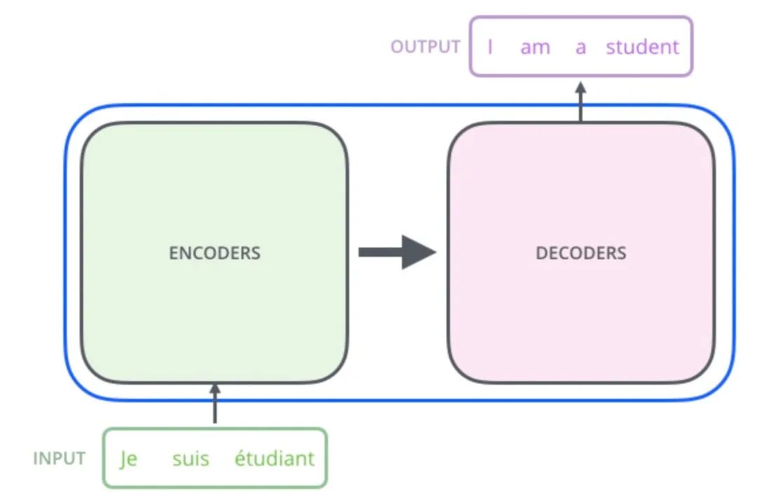
In the OCR recognition task, as shown in the figure below, we hope to recognize the image as “Share”. Essentially, this can also be seen as a sequence-to-sequence task, except that the input sequence information is represented in image form.

Therefore, viewing the OCR problem as a sequence-to-sequence prediction problem makes using transformers to solve OCR problems a very natural and smooth idea. The remaining question is how to structure the information from the image into a format that transformers can use, similar to word embedding.
Returning to our task, since the images to be predicted are all long and the text is mostly horizontally arranged, we will integrate the feature map along the horizontal direction. Each embedding can be regarded as the features of a certain vertical slice of the image, and we will provide such feature sequences to the transformer, utilizing its powerful attention capabilities to complete the predictions.
Thus, based on the above analysis, we define the pipeline of the model framework as shown in the figure below:
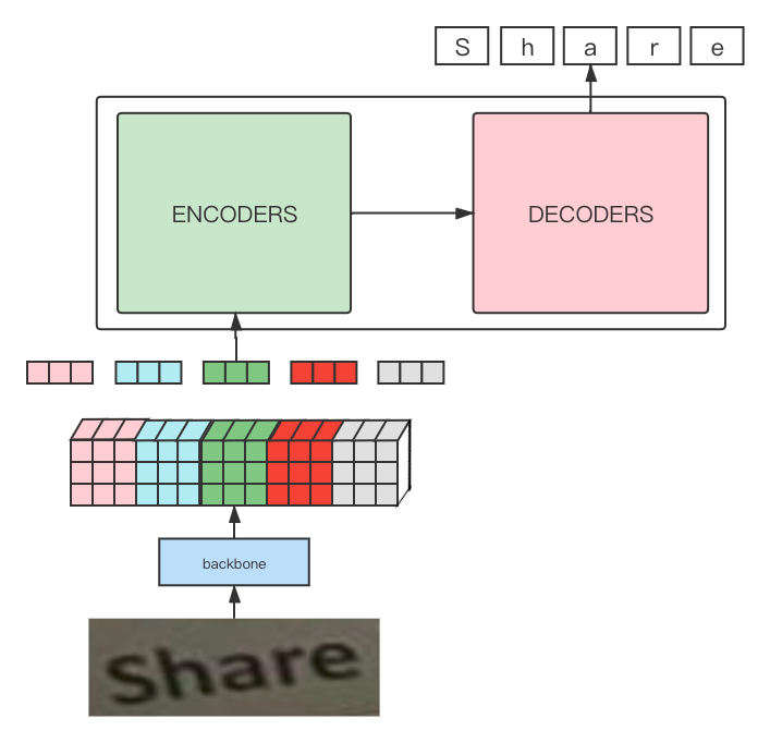
By observing the above figure, it can be found that the entire pipeline is essentially consistent with the process of training transformers for machine translation, with the main difference being the addition of a CNN network as a backbone to extract image features to obtain input embeddings.
The design of constructing the input embedding for the transformer is a key focus of this article and is crucial for the algorithm to work. The following text will elaborate on the relevant details shown in the diagram above in conjunction with the code.
4. Explanation of Training Framework Code
The relevant code for the training framework is implemented in ocr_by_transformer.py
Next, we will gradually explain the code, which mainly consists of the following parts:
-
Constructing the dataset → Image preprocessing, label processing, etc.; -
Model construction → Backbone + Transformer; -
Model training -
Inference → Greedy decoding
Let’s take a look step by step.
4.1 Preparation Work
First, import the libraries needed later.
import os
import time
import copy
from PIL import Image

# Online dataset related packages
from tensorbay import GAS
from tensorbay.dataset import Dataset

# Torch related packages
import torch
import torch.nn as nn
from torch.autograd import Variable
import torchvision.models as models
import torchvision.transforms as transforms

# Import utility class package
from analysis_recognition_dataset import load_lbl2id_map, statistics_max_len_label
from transformer import *
from train_utils import *
Then set some basic parameters.
device = torch.device('cuda')  # 'cpu' or 'cuda'
nrof_epochs = 1500  # Number of iterations, 1500, adjust as needed
batch_size = 64     # Batch size, 64, adjust as needed
model_save_path = './log/ex1_ocr_model.pth'
Online obtain image data and read the character-to-ID mapping dictionary from the image label, which will be used for subsequent Dataset creation.
# GAS credentials
KEY = 'Accesskey-fd26cc098604c68a99d3bf7f87cd480a'
gas = GAS(KEY)
# Online obtaining the dataset
dataset_online = Dataset("ICDAR2015", gas)
dataset_online.enable_cache('./data')  # Enable local cache

# Get training and validation sets
train_data_online = dataset_online["train"]
valid_data_online = dataset_online['valid']

# Read the label-ID mapping relationship record file
lbl2id_map_path = os.path.join('./', 'lbl2id_map.txt')
lbl2id_map, id2lbl_map = load_lbl2id_map(lbl2id_map_path)

# Count how many characters are included in the longest label among all labels appearing in the dataset, which is needed for constructing gt (ground truth) information
train_max_label_len = statistics_max_len_label(train_data_online)
valid_max_label_len = statistics_max_len_label(valid_data_online)
# The case with the most characters in the dataset as the sequence_len for constructing gt
sequence_len = max(train_max_label_len, valid_max_label_len)
4.2 Dataset Construction
Next, let’s introduce the content related to dataset construction. First, consider how to reasonably preprocess the images. Image Preprocessing Scheme
Assuming the image size is
After passing through the network, the feature map size is
Based on the previous analysis of the dataset, the images are mostly horizontal long strips, and the image content consists of horizontally arranged characters that form words. Therefore, the vertical resolution does not need to be very high since the same vertical slice position in the image space generally contains only one character. Thus, a resolution of is sufficient; however, the horizontal resolution needs to be larger as we need different embeddings to encode the features of different characters in the horizontal direction.
Here, we use the classic ResNet-18 network as the backbone. Since its downsampling factor is 32 and the number of channels in the last layer feature map is 512, then:
How to determine the input image width? Here are two options:
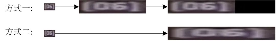
Method 1: Set a fixed size, keeping the image’s aspect ratio during resizing, and padding the right empty area;
Method 2: Directly force the original image to resize to a preset fixed size.
Note: Here, you might want to think about which scheme you think is better?
The author chose Method 1 because the aspect ratio of the images and the number of characters in the words in the images are roughly proportional. If the original aspect ratio of the images is maintained during preprocessing, then each pixel on the feature map corresponding to the character area of the original image will be essentially stable, which may yield better prediction results.
There is also a detail: You will notice in the above image that in each area with a width:height ratio of 1:1, there are generally 2-3 characters distributed. Therefore, in practical operations, we do not strictly maintain the aspect ratio unchanged, but instead increased the aspect ratio by 3 times, that is, we first stretched the original image width to 3 times its original size, and then resized the height to 32 while maintaining the aspect ratio.
Note: Here, it is advisable to stop and think about why this detail is necessary?
The purpose of doing this is to ensure that each character on the image has at least one pixel on the feature map corresponding to it, instead of one pixel on the width dimension of the feature map encoding the information of multiple characters in the original image, which I believe would unnecessarily complicate the transformer’s predictions (this is just a personal view, and discussion is welcome).
Having determined the resizing scheme, what specific settings should we use? Combining the two important indicators from our previous analysis of the dataset, the longest character count in the dataset labels is 21, and the longest aspect ratio is 8.6. We will set the final aspect ratio to 24:1. Thus, summarizing the settings for each parameter:
Related code implementation:
# ----------------
# Image Preprocessing
# ----------------
# Load image
with img_data.open() as fp:
    img = Image.open(fp).convert('RGB')

# Perform roughly proportionate scaling on the image
# Resize height to 32, width roughly proportionately scaled but must be divisible by 32
w, h = img.size
ratio = round((w / h) * 3)   # Stretch width to 3 times its original size, then round
if ratio == 0:
    ratio = 1
if ratio > self.max_ratio:
    ratio = self.max_ratio
h_new = 32
w_new = h_new * ratio
img_resize = img.resize((w_new, h_new), Image.BILINEAR)

# Padding the right half of the image to fix the width/height ratio = self.max_ratio
img_padd = Image.new('RGB', (32*self.max_ratio, 32), (0,0,0))
img_padd.paste(img_resize, (0, 0))
Image Augmentation
Image augmentation is not the focus. Here, in addition to the aforementioned resizing scheme, we perform regular random color transformations and normalization operations on the images.
Complete Code
The complete code for constructing the dataset is as follows:
class Recognition_Dataset(object):

    def __init__(self, segment, lbl2id_map, sequence_len, max_ratio, pad=0):        self.data = segment
        self.lbl2id_map = lbl2id_map
        self.pad = pad   # Padding identifier ID, default 0
        self.sequence_len = sequence_len    # Sequence length
        self.max_ratio = max_ratio * 3      # Stretch the width to 3 times

        # Define random color transformation
        self.color_trans = transforms.ColorJitter(0.1, 0.1, 0.1)
        # Define Normalize
        self.trans_Normalize = transforms.Compose([
            transforms.ToTensor(),
            transforms.Normalize([0.485,0.456,0.406], [0.229,0.224,0.225]),
        ])

    def __getitem__(self, index):
        """
        Get the corresponding index's image and ground truth label, and perform data augmentation if necessary
        """
        img_data = self.data[index]
        lbl_str = img_data.label.classification.category  # Image label

        # ----------------
        # Image Preprocessing
        # ----------------
        # Load image
        with img_data.open() as fp:
            img = Image.open(fp).convert('RGB')

        # Perform roughly proportionate scaling on the image
        # Resize height to 32, width roughly proportionately scaled but must be divisible by 32
        w, h = img.size
        ratio = round((w / h) * 3)   # Stretch width to 3 times its original size, then round
        if ratio == 0:
            ratio = 1
        if ratio > self.max_ratio:
            ratio = self.max_ratio
        h_new = 32
        w_new = h_new * ratio
        img_resize = img.resize((w_new, h_new), Image.BILINEAR)

        # Padding the right half of the image to fix the width/height ratio = self.max_ratio
        img_padd = Image.new('RGB', (32*self.max_ratio, 32), (0,0,0))
        img_padd.paste(img_resize, (0, 0))

        # Random color transformation
        img_input = self.color_trans(img_padd)
        # Normalize
        img_input = self.trans_Normalize(img_input)

        # ----------------
        # Label Processing
        # ----------------

        # Construct encoder's mask
        encode_mask = [1] * ratio + [0] * (self.max_ratio - ratio)
        encode_mask = torch.tensor(encode_mask)
        encode_mask = (encode_mask != 0).unsqueeze(0)

        # Construct ground truth label
        gt = []
        gt.append(1)    # First add the sentence start symbol
        for lbl in lbl_str:
            gt.append(self.lbl2id_map[lbl])
        gt.append(2)
        for i in range(len(lbl_str), self.sequence_len):   # Excluding start and end symbols, lbl length is sequence_len, remaining positions are padded
            gt.append(0)
        # Truncate to the preset maximum sequence length
        gt = gt[:self.sequence_len]

        # Decoder input
        decode_in = gt[:-1]
        decode_in = torch.tensor(decode_in)
        # Decoder output
        decode_out = gt[1:]
        decode_out = torch.tensor(decode_out)
        # Decoder mask
        decode_mask = self.make_std_mask(decode_in, self.pad)
        # Effective tokens count
        ntokens = (decode_out != self.pad).data.sum()

        return img_input, encode_mask, decode_in, decode_out, decode_mask, ntokens

    @staticmethod
    def make_std_mask(tgt, pad):
        """
        Create a mask to hide padding and future words.
        Padding and future words are represented with 0 in the mask.
        """
        tgt_mask = (tgt != pad)
        tgt_mask = tgt_mask & Variable(subsequent_mask(tgt.size(-1)).type_as(tgt_mask.data))
        tgt_mask = tgt_mask.squeeze(0)   # The subsequent return value's shape is (1, N, N)
        return tgt_mask

    def __len__(self):
        return len(self.data)
In the above code, several details related to label processing are involved, which belong to the logic related to transformer training. Here, I will briefly mention them:
encode_mask
Since we adjusted the size of the images and added padding as needed, the padding positions do not contain meaningful information. Therefore, we need to construct the corresponding encode_mask based on the padding ratio to allow the transformer to ignore this meaningless area during computation.
Label Processing
The predicted labels used in this experiment are basically consistent with the labels used during the training of machine translation models, so the differences in processing are relatively small.
In label processing, the characters in the label are converted to their corresponding IDs, the start symbol is added to the beginning of the sentence, the end symbol is added to the end of the sentence, and when the length does not meet the sequence_len, padding (0) is performed in the remaining positions.
decode_mask
In general, in the decoder, we generate an upper triangular matrix mask based on the label’s sequence_len, where each row of the mask can control the current time step to only allow the decoder to obtain information from characters before the current step while prohibiting the acquisition of information from future moments, preventing cheating during model training.
The decode_mask is generated by a special function make_std_mask().
At the same time, the decoder’s label production must also consider masking the padding part, so the decode_mask should also be set to False at the positions corresponding to the padding in the label.
The generated decode_mask is shown in the figure below:

This concludes all the details for constructing the dataset, allowing us to create a DataLoader for training.
# Construct dataloader
max_ratio = 8    # Maximum value of width/height during image preprocessing. If it does not exceed this, keep the aspect ratio during resizing; if it exceeds, force compression.
train_dataset = Recognition_Dataset(train_data_online, lbl2id_map, sequence_len, max_ratio, pad=0)
valid_dataset = Recognition_Dataset(valid_data_online, lbl2id_map, sequence_len, max_ratio, pad=0)
# loader size info:
# --> img_input: [batch_size, c, h, w] --> [64, 3, 32, 32*8*3]
# --> encode_mask: [batch_size, h/32, w/32] --> [64, 1, 24] The backbone used in this article is downsampled by 32, so it is divided by 32.
# --> decode_in: [bs, sequence_len-1] --> [64, 20]
# --> decode_out: [bs, sequence_len-1] --> [64, 20]
# --> decode_mask: [bs, sequence_len-1, sequence_len-1] --> [64, 20, 20]
# --> ntokens: [bs] --> [64]
train_loader = torch.utils.data.DataLoader(train_dataset,
                                        batch_size=batch_size,
                                        shuffle=True,
                                        num_workers=4)
valid_loader = torch.utils.data.DataLoader(valid_dataset,
                                        batch_size=batch_size,
                                        shuffle=False,
                                        num_workers=4)
4.3 Model Construction
The model structure is built through make_ocr_model and OCR_EncoderDecoder classes.
You can start from the make_ocr_model function, which first calls the pretrained ResNet-18 in pytorch as the backbone to extract image features. This can be adjusted to other networks based on your needs, but it is crucial to pay attention to the downsampling factor of the network and the channel number of the last layer feature map, and the parameters of the relevant modules need to be adjusted accordingly. Then, it calls the OCR_EncoderDecoder class to complete the construction of the transformer. Finally, the model parameters are initialized.
In the OCR_EncoderDecoder class, this class serves as an assembly line for the basic components of the transformer, including the encoder and decoder, etc. Its initial parameters are the existing basic components, and the code for these basic components is all in the transformer.py file, which will not be elaborated on here.
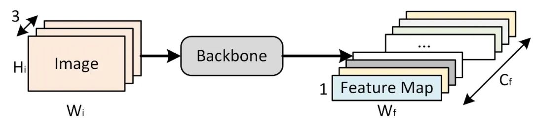
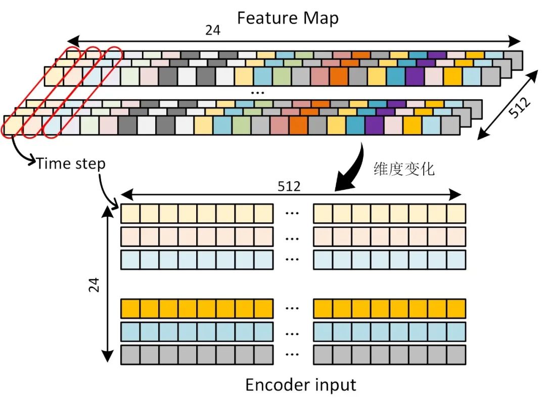
Let’s review how the image passes through the backbone to construct the input for the transformer:
The image passes through the backbone and outputs a feature map with dimensions [batch_size, 512, 1, 24]. Ignoring the batch_size, each image will obtain a feature map with 512 channels and dimensions 1×24, as indicated by the red box in the image. The feature values of the same position from different channels are concatenated to form a new vector, which is used as the input for one time step, thus constructing an input with dimensions [batch_size, 24, 512], meeting the requirements for transformer input.
Next, let’s look at the complete code for constructing the model:
# Model structure
class OCR_EncoderDecoder(nn.Module):
    """
    A standard Encoder-Decoder architecture.
    Base for this and many other models.
    """
    def __init__(self, encoder, decoder, src_embed, src_position, tgt_embed, generator):
        super(OCR_EncoderDecoder, self).__init__()
        self.encoder = encoder
        self.decoder = decoder
        self.src_embed = src_embed    # Input embedding module
        self.src_position = src_position
        self.tgt_embed = tgt_embed    # Output embedding module
        self.generator = generator    # Output generation module

    def forward(self, src, tgt, src_mask, tgt_mask):
        "Take in and process masked src and target sequences."
        # src --> [bs, 3, 32, 768]  [bs, c, h, w]
        # src_mask --> [bs, 1, 24]  [bs, h/32, w/32]
        memory = self.encode(src, src_mask)
        # memory --> [bs, 24, 512]
        # tgt --> decode_in [bs, 20]  [bs, sequence_len-1]
        # tgt_mask --> decode_mask [bs, 20]  [bs, sequence_len-1]
        res = self.decode(memory, src_mask, tgt, tgt_mask)  # [bs, 20, 512]
        return res

    def encode(self, src, src_mask):
        # Feature extract
        # src --> [bs, 3, 32, 768]
        src_embedds = self.src_embed(src)
        # The resnet18 used as the backbone outputs --> [batchsize, c, h, w] --> [bs, 512, 1, 24]
        # Processing src_embedds from shape (bs, model_dim, 1, max_ratio) to the expected input shape (bs, time_step, model_dim)
        # [bs, 512, 1, 24] --> [bs, 24, 512]
        src_embedds = src_embedds.squeeze(-2)
        src_embedds = src_embedds.permute(0, 2, 1)

        # Position encode
        src_embedds = self.src_position(src_embedds)  # [bs, 24, 512]

        return self.encoder(src_embedds, src_mask)  # [bs, 24, 512]

    def decode(self, memory, src_mask, tgt, tgt_mask):
        target_embedds = self.tgt_embed(tgt)  # [bs, 20, 512]
        return self.decoder(target_embedds, memory, src_mask, tgt_mask)


def make_ocr_model(tgt_vocab, N=6, d_model=512, d_ff=2048, h=8, dropout=0.1):
    """
    Construct the model
    params:
        tgt_vocab: Output vocabulary size
        N: Number of basic module stacks in the encoder and decoder
        d_model: Size of embedding in the model, default 512
        d_ff: Size of embedding in FeedForward Layer, default 2048
        h: Number of heads in MultiHeadAttention, must be divisible by d_model
        dropout: Dropout rate
    """
    c = copy.deepcopy

    # The pretrained resnet18 in torch serves as the feature extraction network, backbone
    backbone = models.resnet18(pretrained=True)
    backbone = nn.Sequential(*list(backbone.children())[:-2])    # Remove the last two layers (global average pooling and fc layer)

    attn = MultiHeadedAttention(h, d_model)
    ff = PositionwiseFeedForward(d_model, d_ff, dropout)
    position = PositionalEncoding(d_model, dropout)
 # Construct the model
    model = OCR_EncoderDecoder(
        Encoder(EncoderLayer(d_model, c(attn), c(ff), dropout), N),
        Decoder(DecoderLayer(d_model, c(attn), c(attn), c(ff), dropout), N),
        backbone,
        c(position),
        nn.Sequential(Embeddings(d_model, tgt_vocab), c(position)),
        Generator(d_model, tgt_vocab))  # The generator here is not called within the class

    # Initialize parameters with Glorot / fan_avg.
    for child in model.children():
        if child is backbone:
            # Set the backbone's weights to not compute gradients
            for param in child.parameters():
                param.requires_grad = False
            # The pretrained backbone does not undergo random initialization, while other modules are randomly initialized
            continue
        for p in child.parameters():
            if p.dim() > 1:
                nn.init.xavier_uniform_(p)
    return model
Through the above two classes, we can conveniently construct the transformer model:
# Build model
# Use transformer as OCR recognition model
# The constructed ocr_model does not include the Generator

tgt_vocab = len(lbl2id_map.keys())
d_model = 512
ocr_model = make_ocr_model(tgt_vocab, N=5, d_model=d_model, d_ff=2048, h=8, dropout=0.1)
ocr_model.to(device)
4.4 Model Training
Before training the model, it is also necessary to define the model evaluation criteria, iterative optimizer, etc. In this experiment, label smoothing (label smoothing) and network training warmup strategies are used during training. The calling functions for these strategies are all in train_utils.py, and the principles and code implementations of these two methods will not be discussed here.
Label smoothing can convert the original hard labels into soft labels, thereby increasing the model’s fault tolerance and enhancing its generalization ability. The LabelSmoothing() function in the code implements label smoothing and internally uses the relative entropy function to calculate the loss between predicted and true values.
The warmup strategy can effectively control the learning rate of the optimizer during the model training process, automatically implementing the gradual increase and then decrease of the learning rate, helping the model to be more stable during training and achieving rapid convergence of loss. The NoamOpt() function in the code implements warmup control, using the Adam optimizer to automatically adjust the learning rate with the number of iterations.
# Train prepare
criterion = LabelSmoothing(size=tgt_vocab, padding_idx=0, smoothing=0.0)  # Label smoothing
optimizer = torch.optim.Adam(ocr_model.parameters(), lr=0, betas=(0.9, 0.98), eps=1e-9)
model_opt = NoamOpt(d_model, 1, 400, optimizer)  # Warmup
The code for the model training process is as follows. Validation is performed every 10 epochs, and the calculation process for a single epoch is encapsulated in the run_epoch() function.
# Train & valid ...
for epoch in range(nrof_epochs):
    print(f"\nepoch {epoch}")

    print("train...")  # Training
    ocr_model.train()
    loss_compute = SimpleLossCompute(ocr_model.generator, criterion, model_opt)
    train_mean_loss = run_epoch(train_loader, ocr_model, loss_compute, device)

    if epoch % 10 == 0:
        print("valid...")  # Validation
        ocr_model.eval()
        valid_loss_compute = SimpleLossCompute(ocr_model.generator, criterion, None)
        valid_mean_loss = run_epoch(valid_loader, ocr_model, valid_loss_compute, device)
        print(f"valid loss: {valid_mean_loss}")

        # Save model
        torch.save(ocr_model.state_dict(), './trained_model/ocr_model.pt')
SimpleLossCompute() class implements the loss calculation for the transformer output results. When using this class for direct calculation, it needs to receive three parameters: (x, y, norm), where x is the output from the decoder, y is the label data, and norm is the normalization coefficient for the loss, which can be the number of all effective tokens in the batch. This shows that the complete construction of the transformer network is realized here, achieving the flow of data computation.
run_epoch() function internally completes all work for training one epoch, including data loading, model inference, loss calculation, and direction propagation, while printing the training process information.
def run_epoch(data_loader, model, loss_compute, device=None):
    "Standard Training and Logging Function"
    start = time.time()
    total_tokens = 0
    total_loss = 0
    tokens = 0

    for i, batch in enumerate(data_loader):
        img_input, encode_mask, decode_in, decode_out, decode_mask, ntokens = batch
        img_input = img_input.to(device)
        encode_mask = encode_mask.to(device)
        decode_in = decode_in.to(device)
        decode_out = decode_out.to(device)
        decode_mask = decode_mask.to(device)
        ntokens = torch.sum(ntokens).to(device)

        out = model.forward(img_input, decode_in, encode_mask, decode_mask)
        # out --> [bs, 20, 512]  Prediction results
        # decode_out --> [bs, 20]  Actual results
        # ntokens --> Actual effective characters in the label

        loss = loss_compute(out, decode_out, ntokens)  # Loss calculation
        total_loss += loss
        total_tokens += ntokens
        tokens += ntokens
        if i % 50 == 1:
            elapsed = time.time() - start
            print("Epoch Step: %d Loss: %f Tokens per Sec: %f" %
                    (i, loss / ntokens, tokens / elapsed))
            start = time.time()
            tokens = 0
    return total_loss / total_tokens


class SimpleLossCompute:
    "A simple loss compute and train function."
    def __init__(self, generator, criterion, opt=None):
        self.generator = generator
        self.criterion = criterion
        self.opt = opt

    def __call__(self, x, y, norm):
        """
        norm: Normalization coefficient for the loss, which can be the number of effective tokens in the batch.
        """
        # x --> out --> [bs, 20, 512]  Prediction results
        # y --> decode_out --> [bs, 20]  Actual results
        # norm --> ntokens --> Actual effective characters in the label
        x = self.generator(x)
        # Label smoothing requires corresponding dimensional changes
        x_ = x.contiguous().view(-1, x.size(-1))  # [20bs, 512]
        y_ = y.contiguous().view(-1)  # [20bs]
        loss = self.criterion(x_, y_)
        loss /= norm
        loss.backward()
        if self.opt is not None:
            self.opt.step()
            self.opt.optimizer.zero_grad()
        #return loss.data[0] * norm
        return loss.item() * norm
4.5 Greedy Decoding
For convenience, we use the simplest greedy decoding to directly predict OCR results. Since the model will produce only one output each time, we choose the character corresponding to the highest probability in the output probability distribution as the prediction result for this prediction, and then predict the next character. This is known as greedy decoding, as seen in the greedy_decode() function in the code.
In the experiment, each image is used as the input to the model, and the correct rate is counted through greedy decoding one by one, ultimately providing the prediction accuracy for both the training set and the validation set.
# After training, use the greedy decoding method to infer the training set and validation set, counting the correct rate
ocr_model.eval()

print("\n------------------------------------------------")
print("Greedy decode trainset")
total_img_num = 0
total_correct_num = 0
for batch_idx, batch in enumerate(train_loader):
    img_input, encode_mask, decode_in, decode_out, decode_mask, ntokens = batch
    img_input = img_input.to(device)
    encode_mask = encode_mask.to(device)

    # Get information for a single image
    bs = img_input.shape[0]
    for i in range(bs):
        cur_img_input = img_input[i].unsqueeze(0)
        cur_encode_mask = encode_mask[i].unsqueeze(0)
        cur_decode_out = decode_out[i]
  # Greedy decoding
        pred_result = greedy_decode(ocr_model, cur_img_input, cur_encode_mask, max_len=sequence_len, start_symbol=1, end_symbol=2)
        pred_result = pred_result.cpu()
  # Check if the prediction is correct
        is_correct = judge_is_correct(pred_result, cur_decode_out)
        total_correct_num += is_correct
        total_img_num += 1
        if not is_correct:
            # Print cases of incorrect predictions
            print("----")
            print(cur_decode_out)
            print(pred_result)
        total_correct_rate = total_correct_num / total_img_num * 100
        print(f"Total correct rate of trainset: {total_correct_rate}%")

# The decoding code for the training set is the same
print("\n------------------------------------------------")
print("Greedy decode validset")
total_img_num = 0
total_correct_num = 0
for batch_idx, batch in enumerate(valid_loader):
    img_input, encode_mask, decode_in, decode_out, decode_mask, ntokens = batch
    img_input = img_input.to(device)
    encode_mask = encode_mask.to(device)

    bs = img_input.shape[0]
    for i in range(bs):
        cur_img_input = img_input[i].unsqueeze(0)
        cur_encode_mask = encode_mask[i].unsqueeze(0)
        cur_decode_out = decode_out[i]

        pred_result = greedy_decode(ocr_model, cur_img_input, cur_encode_mask, max_len=sequence_len, start_symbol=1, end_symbol=2)
        pred_result = pred_result.cpu()

        is_correct = judge_is_correct(pred_result, cur_decode_out)
        total_correct_num += is_correct
        total_img_num += 1
        if not is_correct:
            # Print cases of incorrect predictions
            print("----")
            print(cur_decode_out)
            print(pred_result)
        total_correct_rate = total_correct_num / total_img_num * 100
        print(f"Total correct rate of validset: {total_correct_rate}%")
greedy_decode() function is implemented as follows.
# Greedy decode
def greedy_decode(model, src, src_mask, max_len, start_symbol, end_symbol):
    memory = model.encode(src, src_mask)
    # ys represents the currently generated sequence, initially containing only a start symbol, continuously appending the predicted results to the end of the sequence
    ys = torch.ones(1, 1).fill_(start_symbol).type_as(src.data).long()
    for i in range(max_len-1):
        out = model.decode(memory, src_mask,
                           Variable(ys),
                           Variable(subsequent_mask(ys.size(1)).type_as(src.data)))
        prob = model.generator(out[:, -1])
        _, next_word = torch.max(prob, dim = 1)
        next_word = next_word.data[0]
        next_word = torch.ones(1, 1).type_as(src.data).fill_(next_word).long()
        ys = torch.cat([ys, next_word], dim=1)

        next_word = int(next_word)
        if next_word == end_symbol:
            break
        #ys = torch.cat([ys, torch.ones(1, 1).type_as(src.data).fill_(next_word)], dim=1)
    ys = ys[0, 1:]
    return ys


def judge_is_correct(pred, label):
    # Determine whether the model's prediction result is consistent with the label
    pred_len = pred.shape[0]
    label = label[:pred_len]
    is_correct = 1 if label.equal(pred) else 0
    return is_correct
Run the command below to start training with one click:
python ocr_by_transformer.py
The training log is as follows:
epoch 0
train...
Epoch Step: 1 Loss: 5.142612 Tokens per Sec: 852.649109
Epoch Step: 51 Loss: 3.064528 Tokens per Sec: 2709.471436
valid...
Epoch Step: 1 Loss: 3.018526 Tokens per Sec: 1413.900391
valid loss: 2.7769546508789062

epoch 1
train...
Epoch Step: 1 Loss: 3.440590 Tokens per Sec: 1303.567993
Epoch Step: 51 Loss: 2.711708 Tokens per Sec: 2743.414307
...
epoch 1499
train...
Epoch Step: 1 Loss: 0.005739 Tokens per Sec: 1232.602783
Epoch Step: 51 Loss: 0.013249 Tokens per Sec: 2765.866211

------------------------------------------------
greedy decode trainset
----
tensor([17, 32, 18, 19, 31, 50, 30, 10, 30, 10, 17, 32, 41, 55, 55, 55,  2,  0,
         0,  0])
tensor([17, 32, 18, 19, 31, 50, 30, 10, 30, 10, 17, 32, 41, 55, 55, 55, 55, 55,
        55, 55])
----
tensor([17, 32, 18, 19, 31, 50, 30, 10, 17, 32, 41, 55, 55,  2,  0,  0,  0,  0,
         0,  0])
tensor([17, 32, 18, 19, 31, 50, 30, 10, 17, 32, 41, 55, 55, 55, 55,  2])
total correct rate of trainset: 99.95376791493297%

------------------------------------------------
greedy decode validset
----
tensor([10, 11, 28, 27, 25, 11, 47, 45,  2,  0,  0,  0,  0,  0,  0,  0,  0,  0,
         0,  0])
tensor([10, 11, 28, 27, 25, 11, 62,  2])

...
tensor([20, 12, 24, 35,  2,  0,  0,  0,  0,  0,  0,  0,  0,  0,  0,  0,  0,  0,
         0,  0])
tensor([20, 12, 21, 12, 22, 23, 34,  2])
total correct rate of validset: 92.72088353413655%
Summary
This concludes the entire content of this article. Congratulations on reading this far !
!
In this article, we first introduced a word recognition task dataset from ICDAR2015, then conducted a simple analysis of the data characteristics, and constructed a character mapping relationship table for recognition. After that, we focused on introducing the motivation and ideas for integrating transformers to solve OCR tasks, detailing the details in conjunction with the code, and finally briefly went over some training-related logic and code.
This article mainly aims to help everyone broaden their thinking and understand other application points of transformers in CV beyond serving as backbones. The implementation code for the transformer model itself refers to The Annotated Transformer, while the application to the OCR part is entirely based on the author’s personal understanding and implementation, and it cannot be guaranteed to be applicable to more complex engineering problems. If there are any details in the article that you have questions about, please feel free to contact us for discussion, and if there are any errors, please kindly point them out.
We hope you gain something from reading this!
Good news!
The Visual Learning for Beginners knowledge circle is now open to the public👇👇👇


Download 1: OpenCV-Contrib Extension Module Chinese Version Tutorial
Reply "Extension Module Chinese Tutorial" in the background of the "Visual Learning for Beginners" public account to download the first Chinese version of the OpenCV extension module tutorial on the internet, covering over twenty chapters including extension module installation, SFM algorithms, stereo vision, target tracking, biological vision, super-resolution processing, etc.

Download 2: Python Vision Practical Project 52 Lectures
Reply "Python Vision Practical Project" in the background of the "Visual Learning for Beginners" public account to download 31 visual practical projects including image segmentation, mask detection, lane line detection, vehicle counting, eyeliner addition, license plate recognition, character recognition, emotion detection, text content extraction, face recognition, etc., to help quickly learn computer vision.

Download 3: OpenCV Practical Projects 20 Lectures
Reply "OpenCV Practical Projects 20 Lectures" in the background of the "Visual Learning for Beginners" public account to download 20 practical projects based on OpenCV, achieving advanced learning of OpenCV.

Discussion Group

You are welcome to join the reader group of the public account to communicate with peers. Currently, there are WeChat groups for SLAM, 3D vision, sensors, autonomous driving, computational photography, detection, segmentation, recognition, medical imaging, GAN, algorithm competitions, etc. (these will be gradually subdivided in the future). Please scan the WeChat number below to join the group, and note: "Nickname + School/Company + Research Direction", for example: "Zhang San + Shanghai Jiao Tong University + Visual SLAM". Please follow the format for notes, otherwise it will not be approved. After successfully adding, you will be invited to the relevant WeChat group based on your research direction. Please do not send advertisements in the group, otherwise you will be removed from the group. Thank you for your understanding~