Click the "Advanced Programming" above and select the "Star" public accountSuper valuable content delivered to you immediately!!!

In this article, we will demonstrate how to build a simple three-layer neural network from scratch. Although we will not derive all the mathematical operations involved in detail, I will do my best to explain our approach intuitively.
Here, I assume you have a basic understanding of calculus and concepts in machine learning, such as classification and regularization. It would be best if you also understand the principles of optimization techniques like gradient descent. However, even if you are not very familiar with these topics, this article will still be interesting!
So, why implement a neural network from scratch? Even if you plan to use a neural network library like PyBrain in the future, implementing a network from scratch at least once is a very valuable exercise. It helps you understand how neural networks work, which is crucial for designing effective models.
Generating the Dataset
Let’s start by generating a usable dataset. Fortunately, scikit-learn has some useful dataset generators, so we don’t need to write the code ourselves. We will use the make_moons function.
# Generate a dataset and plot it
np.random.seed(0)
X, y = sklearn.datasets.make_moons(200, noise=0.20)
plt.scatter(X[:,0], X[:,1], s=40, c=y, cmap=plt.cm.Spectral)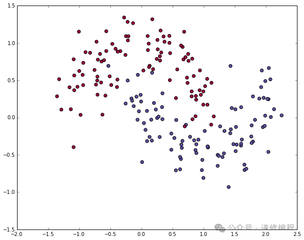
The dataset we generated has two classes, plotted as red and blue dots. You can think of the blue dots as male patients and the red dots as female patients, with the x-axis and y-axis representing medical measurements.
Our goal is to train a machine learning classifier that predicts the correct class (male or female) given the x and y coordinates. Note that the data is not linearly separable, and we cannot draw a straight line to separate the two classes. This means that linear classifiers (like logistic regression) will not fit the data unless you manually design nonlinear features suitable for the given dataset (like polynomials).
In fact, this is one of the main advantages of neural networks. You don’t have to worry about feature engineering. The hidden layers of the neural network will learn the features for you.
Logistic Regression
To demonstrate this, let’s train a logistic regression classifier. Its inputs will be the x and y values, and the output will be the predicted class (0 or 1). To make our lives easier, we used the logistic regression class from scikit-learn.
# Train the logistic regression classifier
clf = sklearn.linear_model.LogisticRegressionCV()
clf.fit(X, y)
# Plot the decision boundary
plot_decision_boundary(lambda x: clf.predict(x))
plt.title("Logistic Regression")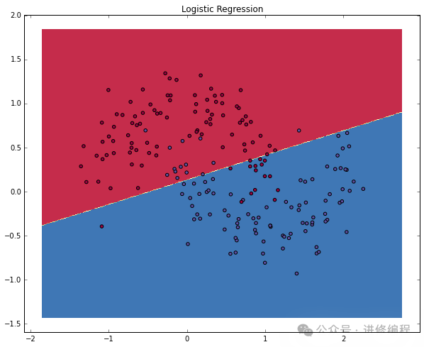
The figure shows the decision boundary learned by our logistic regression classifier. It uses a straight line to separate the data as best as possible, but it cannot capture the “moon shape” of our data.
Training the Neural Network
Now let’s build a three-layer neural network with an input layer, a hidden layer, and an output layer. The number of nodes in the input layer is determined by the dimensionality of the data, which is 2. Similarly, the number of nodes in the output layer is determined by the number of classes we have, which is also 2. (Since we only have 2 classes, we could actually use just one output node to predict 0 or 1, but having 2 makes it easier to extend the network to more classes). The input to the network will be the x and y coordinates, and its output will be two probabilities, one for class 0 (“female”) and the other for class 1 (“male”). It looks like this:
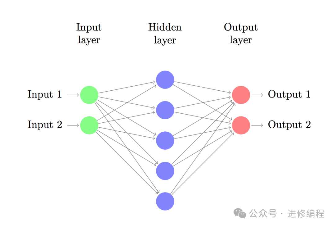
We can choose the dimensionality (number of nodes) of the hidden layer. The more nodes we place in the hidden layer, the more complex the functions we can fit. But higher dimensionality comes at a cost. First, more computation is needed to make predictions and learn the network parameters. More parameters also mean we are more prone to overfitting our data.
How do we choose the size of the hidden layer? While there are some general guidelines and recommendations, it always depends on your specific problem, more of an art than a science. Later, we will discuss the number of nodes in the hidden layer and see how it affects our output.
We also need to choose an activation function for the hidden layer. The activation function converts the inputs of the layer into its outputs. Nonlinear activation functions allow us to fit nonlinear hypotheses. Common choices for activation functions are tanh, sigmoid function, or ReLUs. We will use tanh, which performs quite well in many cases. A good property of these functions is that their derivatives can be computed using the raw function values.
Since we want our network to output probabilities, the activation function for the output layer will be softmax, which is a way to convert raw scores into probabilities. If you are familiar with logistic functions, you can think of softmax as a generalization of it to multiple classes.
How Our Network Makes Predictions
Our network makes predictions using forward propagation, which is just a bunch of matrix multiplications and the application of the activation functions we defined above. If x is the two-dimensional input to our network, we compute our predictions as follows:
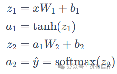
 are the parameters of our network that we need to learn from the training data. You can think of them as matrices that transform data between the layers of the network. Looking at the matrix multiplications above, we can calculate the dimensions of these matrices. If we use 500 nodes in the hidden layer, then:

Now you understand why if we increase the size of the hidden layer, we will have more parameters.
Learning the network parameters means finding the parameters (W1, b1, W2, b2) that minimize the error on the training data. But how do we define error? We use a loss function to measure the error. In softmax output, a common choice is the categorical cross-entropy loss (also known as negative log likelihood). For N training examples and C classes, our prediction loss L(y, y^) relative to the true labels y can be calculated using the following formula:
L(y, y^) = – (1/N) * sum(sum(y_n,i * log(y^_n,i)))
Although this formula looks complex, it is actually just a summation over our training examples, where the loss increases if our predicted classes are incorrect. The larger the difference between the probability distributions of the true labels y and the predicted y^, the larger the loss. By finding the parameters that minimize the loss, we can maximize the likelihood of the training data.
We can use gradient descent to find this minimum. We will implement the simplest version of gradient descent, which is batch gradient descent with a fixed learning rate. In practice, variants like SGD (stochastic gradient descent) or mini-batch gradient descent usually perform better. So, if you are very serious, you might consider using one of these and gradually decreasing the learning rate during training.
Gradient descent requires the gradient (derivative vector) of the loss function with respect to the parameters as input:
-
dL/dW1: The gradient of the loss function with respect to W1
-
dL/db1: The gradient of the loss function with respect to b1
-
dL/dW2: The gradient of the loss function with respect to W2
-
dL/db2: The gradient of the loss function with respect to b2
To compute these gradients, we use the famous backpropagation algorithm, which is an efficient way to compute gradients by propagating backward from the output. I won’t go into detail about how backpropagation works, but there are many great resources online explaining it (like here or here).
Applying the backpropagation formulas, we get the following results (just trust these results):
-
δ3 = y^ – y
-
δ2 = (1 – tanh^2(z1)) ∘ (δ3 * W2^T)
-
dL/dW2 = a1^T * δ3
-
dL/db2 = δ3
-
dL/dW1 = x^T * δ2
-
dL/db1 = δ2
Implementation
Now we are ready to implement it. First, let’s define some useful variables and parameters for gradient descent
num_examples = len(X)  # training set size
n_input_dim = 2  # input layer dimensionality
n_output_dim = 2  # output layer dimensionality
# Gradient descent parameters (I picked these by hand)
epsilon = 0.01  # learning rate for gradient descent
reg_lambda = 0.01  # regularization strength
First, let’s implement the loss function we defined above. We use it to evaluate how our model is performing:
# Helper function to evaluate the total loss on the dataset
def calculate_loss(model):
    W1, b1, W2, b2 = model['W1'], model['b1'], model['W2'], model['b2']
    # Forward propagation to calculate our predictions
    z1 = X.dot(W1) + b1
    a1 = np.tanh(z1)
    z2 = a1.dot(W2) + b2
    exp_scores = np.exp(z2)
    probs = exp_scores / np.sum(exp_scores, axis=1, keepdims=True)
    # Calculating the loss
    correct_logprobs = -np.log(probs[range(num_examples), y])
    data_loss = np.sum(correct_logprobs)
    # Add regularization term to loss (optional)
    data_loss += reg_lambda/2 * (np.sum(np.square(W1)) + np.sum(np.square(W2)))
    return 1./num_examples * data_loss
We also implemented a helper function to calculate the network’s output. It performs the forward propagation defined above and returns the class with the highest probability.
# Helper function to predict an output (0 or 1)
def predict(model, x):
    W1, b1, W2, b2 = model['W1'], model['b1'], model['W2'], model['b2']
    # Forward propagation
    z1 = x.dot(W1) + b1
    a1 = np.tanh(z1)
    z2 = a1.dot(W2) + b2
    exp_scores = np.exp(z2)
    probs = exp_scores / np.sum(exp_scores, axis=1, keepdims=True)
    return np.argmax(probs, axis=1)
Finally, here is the function to train our neural network. It uses the backpropagation derivatives we found above to implement batch gradient descent.
# This function learns parameters for the neural network and returns the model.
# - nn_hdim: Number of nodes in the hidden layer
# - num_passes: Number of passes through the training data for gradient descent
# - print_loss: If True, print the loss every 1000 iterations
def build_model(nn_hdim, num_passes=20000, print_loss=False):
    # Initialize the parameters to random values. We need to learn these.
    np.random.seed(0)
    W1 = np.random.randn(nn_input_dim, nn_hdim) / np.sqrt(nn_input_dim)
    b1 = np.zeros((1, nn_hdim))
    W2 = np.random.randn(nn_hdim, nn_output_dim) / np.sqrt(nn_hdim)
    b2 = np.zeros((1, nn_output_dim))
    # This is what we return at the end
    model = {}
    # Gradient descent. For each batch...
    for i in xrange(0, num_passes):
        # Forward propagation
        z1 = X.dot(W1) + b1
        a1 = np.tanh(z1)
        z2 = a1.dot(W2) + b2
        exp_scores = np.exp(z2)
        probs = exp_scores / np.sum(exp_scores, axis=1, keepdims=True)
        # Backpropagation
        delta3 = probs
        delta3[range(num_examples), y] -= 1
        dW2 = (a1.T).dot(delta3)
        db2 = np.sum(delta3, axis=0, keepdims=True)
        delta2 = delta3.dot(W2.T) * (1 - np.power(a1, 2))
        dW1 = np.dot(X.T, delta2)
        db1 = np.sum(delta2, axis=0)
        # Add regularization terms (b1 and b2 don't have regularization terms)
        dW2 += reg_lambda * W2
        dW1 += reg_lambda * W1
        # Gradient descent parameter update
        W1 += -epsilon * dW1
        b1 += -epsilon * db1
        W2 += -epsilon * dW2
        b2 += -epsilon * db2
        # Assign new parameters to the model
        model = { 'W1': W1, 'b1': b1, 'W2': W2, 'b2': b2}
        # Optionally print the loss.
        # This is expensive because it uses the whole dataset, so we don't want to do it too often.
        if print_loss and i % 1000 == 0:
            print "Loss after iteration %i: %f" %(i, calculate_loss(model))
    return model
Network with Hidden Layer Size of 3
Let’s see what happens if we train a network with a hidden layer size of 3
# Build a model with a 3-dimensional hidden layer
model = build_model(3, print_loss=True)
# Plot the decision boundary
plot_decision_boundary(lambda x: predict(model, x))
plt.title("Decision Boundary for hidden layer size 3")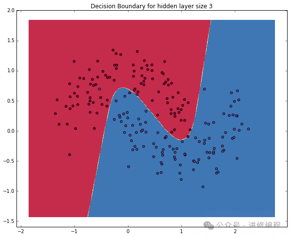
Yay! This looks good. Our neural network is able to find a decision boundary that successfully separates the classes.
Changing Hidden Layer Size
In the example above, we chose a hidden layer size of 3. Now let’s explore how changing the hidden layer size affects the results
plt.figure(figsize=(16, 32))
hidden_layer_dimensions = [1, 2, 3, 4, 5, 20, 50]
for i, nn_hdim in enumerate(hidden_layer_dimensions):
    plt.subplot(5, 2, i+1)
    plt.title('Hidden Layer size %d' % nn_hdim)
    model = build_model(nn_hdim)
    plot_decision_boundary(lambda x: predict(model, x))
plt.show()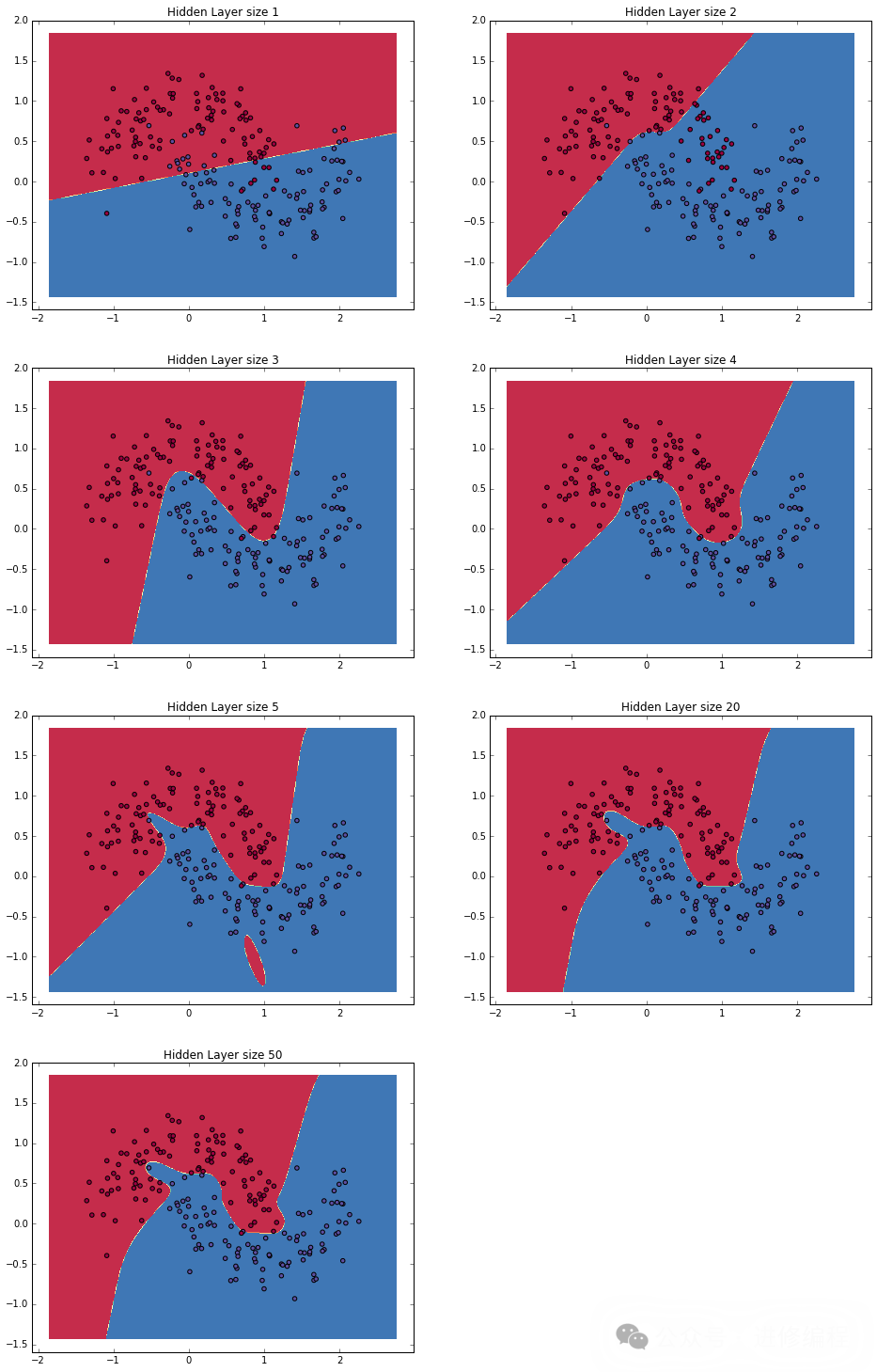
— The End —