Image Recognition Method for Wolframite Based on Deep Learning

Image recognition of wolframite is an efficient way to replace manual selection and waste disposal in wolframite beneficiation, but there is a problem of not being able to distinguish between wolframite ore and surrounding rock waste. This paper uses transfer learning with Convolutional Neural Networks (CNN) in deep learning to solve this problem. This method has the advantages of fast convergence, small required dataset, and high classification accuracy. First, data augmentation methods such as rotation and translation are applied to the colored images of wolframite ore to reduce sample imbalance. Secondly, a new training is conducted using the optimized neural network based on the Keras framework. The results show that in the recognition of two categories, wolframite ore and surrounding rock, the Wu-VGG19 transfer network achieved the highest recognition rate of 97.51%. Additionally, this paper includes the category of quartz gangue in further experiments, resulting in the modified Wu-v3 transfer network achieving the highest recognition rate of 99.6%.

Wolframite beneficiation generally adopts a combined process mainly based on gravity separation, as shown in Fig. 1. The rough selection method for wolframite has been continuously improved, evolving from a single manual selection method to a multi-method combined process, including photoelectric, dense medium separation, and dynamic screening jigging methods. However, due to its economic and technical effectiveness not being superior to manual selection, over 60% of tungsten mines in China still rely on manual selection and waste disposal.

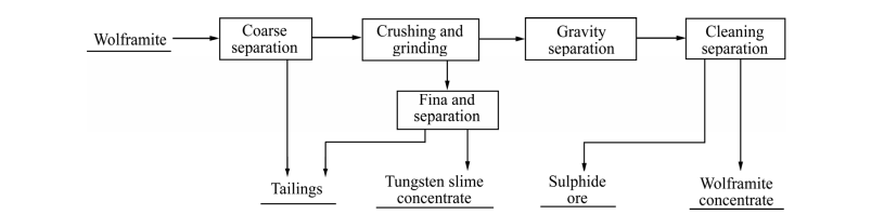
Fig. 1 General flow of wolframite beneficiation

Fig. 1 General flow of wolframite beneficiation

Since the 1990s, machine learning has begun to be applied in the mining industry. In terms of beneficiation, Patel et al. used a machine vision-based Support Vector Machine (SVM) algorithm to classify iron ore of different grades, achieving a classification error rate of only 0.27%. However, this model’s effectiveness heavily relies on features provided by humans, necessitating manual feature extraction strategies, resulting in a cumbersome preprocessing process; Singh et al. classified the feed ore of a ferromanganese smelting plant using a Radial Basis Neural Network based on images, achieving an accuracy of 88.71%; Ebrahimi et al. proposed a computer vision method based on Analytic Hierarchy Process and feature mapping to identify 16 common ores. Wei Lixin et al. introduced a multilayer perceptron rolling force forecasting model based on deep learning, which reduced the relative error between network predictions and measured data to below 3%, achieving high-precision rolling force predictions. Tian Qinghua et al. simulated the antimony leaching process using an Artificial Neural Network model, achieving a correlation coefficient of 99% between experimental and predicted values. Zheng Weida et al. predicted four performance parameters of perovskite material datasets using different machine learning algorithms. In summary, traditional rough selection processes for tungsten ore are costly and difficult to popularize, while existing image-based automatic recognition technologies involve cumbersome preprocessing and low accuracy, making it challenging to balance efficiency and cost. In recent years, deep learning has achieved remarkable results in the field of image recognition, with deep convolutional neural networks such as AlexNet, GoogleNet, and ResNet exceeding human accuracy in certain recognition tasks in the ImageNet Large Scale Visual Recognition Challenge (ILSVRC). The core of these networks is to learn features from raw data for subsequent classification without prior feature engineering, such as manually designing feature contents or quantities. ImageNet contains over 20,000 categories, and the challenge selects 1,000 non-overlapping classes for recognition tasks. A significant breakthrough was achieved in solving the ImageNet challenge in 2012, widely regarded as the beginning of the deep learning revolution of 2010. Convolutional Neural Networks (CNN) are one of the important algorithms in deep learning, theoretically capable of capturing abstract features in images as the number of network layers increases. However, CNNs can easily fall into overfitting with small sample data, and transfer learning is one of the effective approaches to address this issue.

Transfer Learning aims to apply knowledge or patterns learned in one domain or task to a different but related domain or task. This method attempts to achieve the human ability to learn through analogy, such as using skills learned from riding a bicycle to learn how to ride a motorcycle. Transfer learning is widely applicable; for example, Wang et al. used transfer learning with AlexNet to recognize 20 types of vehicles; Dai et al. proposed a translation transfer learning method to help classify images using textual data. In engineering applications, collecting sufficient labeled data for each application domain is often prohibitively expensive or even impossible, making it crucial to transfer existing knowledge from similar domains or tasks to complete or improve target tasks. Therefore, transfer learning can be considered an efficient method for conducting machine learning with minimal human supervision costs. Based on the aforementioned research, this paper addresses the issue of the inability to effectively distinguish between wolframite ore and surrounding rock waste in image recognition methods for wolframite by utilizing pre-trained CNNs for transfer learning to complete the recognition task. First, to reduce sample imbalance, data augmentation methods such as rotation, translation, and noise addition are applied to the RGB images of the wolframite dataset; secondly, under the Keras framework, the optimized VGG19, Inception-V3, InceptionResnet-V2, and InceptionResnet-50 CNNs are used to conduct transfer learning experiments on the dataset; finally, to further recognize the significant grade differences between the two types of ores, the category of quartz gangue is added to the dataset for further experimentation, aiming to have significant practical implications for improving the wolframite beneficiation process.

(1) Dataset Collection

Image samples were collected from three tungsten mines in China. The raw wolframite ore can be mainly divided into three categories: surrounding rock, tungsten ore, and quartz. The samples were taken from different particle sizes of raw ore transported by the manual selection belt in the beneficiation plant (after water washing), placing randomly selected raw ore on the belt surface (with sufficient indoor lighting), and then using a 12-megapixel smartphone to photograph the original samples from different angles at a distance of about 10 cm. A total of approximately 2,500 images were captured, manually divided into three categories: 900 images of black surrounding rock, 210 images of tungsten ore, and 1,400 images of quartz. Due to the limitations of shooting conditions, the sample dataset is too small and imbalanced, significantly affecting recognition accuracy.

(2) Image Data Augmentation

To reduce sample imbalance and address the issue of model overfitting caused by a small dataset, data augmentation operations are performed on the training samples to improve the classification accuracy of the transfer network. Common data augmentation methods include adjustments to image brightness, saturation, contrast, PCA jitter, scaling transformations, image cropping, resizing, horizontal/vertical flipping, translation/rotation/affine transformations, and adding Gaussian noise or blur processing. Different augmentation methods can be selected for different sample sets. In this paper, after preprocessing the samples by cropping, the samples are rotated (45°, 135°), translated, scaled (1.5 times, 0.5 times, and 0.25 times), horizontally/vertically flipped, and random noise is added. Through these data augmentation methods, each category of the dataset reaches 1,500 images. Considering that stable lighting can be provided during actual recognition, brightness, saturation, and contrast adjustment methods were not used.

(1) Experimental Principles

Convolutional Neural Networks have long been one of the core algorithms in the field of image recognition and have shown stable performance when learning from large amounts of data. They can be used to extract discriminative features from images for other classifiers to learn from. Feature extraction can be done by manually inputting different parts of the image into the network or can be extracted by the network itself through unsupervised learning.

Convolutional Neural Networks use deep network structures to extract high-dimensional abstract features from images, completing image recognition and classification tasks. The convolution kernels in the hidden layers have parameter sharing and sparsity in inter-layer connections, allowing the network to learn grid (pixel and audio) data with a relatively small amount of computation, resulting in stable performance without additional feature engineering. The structure of a Convolutional Neural Network generally consists of an input layer, hidden layers (convolutional layers, pooling layers, fully connected layers), and an output layer, as shown in Fig. 2.

1) Input Layer: Since CNNs use gradient descent for learning, input features need to be standardized. For example, input pixel data can be normalized from the original pixel values [0,255] to the range [0,1]. Standardizing input features helps improve the efficiency of the algorithm and learning performance.

2) Convolutional Layer: The convolutional layer is responsible for feature extraction from input data. It contains multiple convolution kernels, with each element of the convolution kernel corresponding to a weight coefficient (W) and a bias (b). Each neuron in the layer is connected to multiple neighboring neurons in the previous layer, with the number of connections determined by the size of the convolution kernel, referred to as the receptive field, which is conceptually similar to the receptive fields of visual cortex cells. When the convolution kernel operates, it systematically scans the input features, performing matrix element multiplication and summing them within the receptive field, and adding the bias.

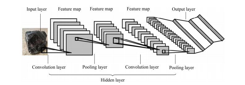
Fig. 2 General structure of convolutional neural networks

Fig. 2 General structure of convolutional neural networks

3) Activation Layer: Its function is to process the linear output from the previous layer through a nonlinear activation function to enhance the network’s representational ability. Activation functions include Sigmoid, Tanh, ReLU, etc.

4) Pooling Layer: After the convolutional layer extracts feature maps, the feature maps are sent to the pooling layer for information filtering and feature selection. The pooling function within the pooling layer calculates the statistical characteristics of the feature map in the neighboring area of a single point. The pooling layer selects the pooling region in the same manner as the convolution kernel scans the feature map, controlled by pooling size, stride, and padding. Based on local correlations, pooling retains useful information while reducing data scale; pooling also possesses local linear transformation invariance, enhancing the generalization ability of Convolutional Neural Networks.

5) Fully Connected Layer: The fully connected layer is usually located at the end of the hidden layers of the Convolutional Neural Network, passing signals only to other fully connected layers. The three-dimensional feature maps are flattened into a one-dimensional vector in the fully connected layer and passed to the next layer through an activation function.

6) Output Layer: The upstream of the output layer in a Convolutional Neural Network is typically a fully connected layer, so its structure and operation are the same as those of the output layer in traditional feedforward neural networks. For image classification problems, the output layer uses a logistic function or a normalized exponential function (Softmax function) to output classification labels.

(2) Experimental Methods

This paper adopts an image recognition method based on transfer learning to identify ores, as shown in Fig. 3(a). The pre-trained network’s neuron connection structure is very complex; Fig. 3(a) shows a simplified structure of the pre-trained network. Fig. 3(b) shows the fully connected layer structure designed in this paper. The connection form of each neuron in the second and third layers is the same as that of the first neuron in each layer, with the last layer having three neurons corresponding to the three ore category labels. For example, when the output result is [0,1,0], it indicates the identified category is tungsten ore. First, the weight file is loaded to initialize network parameters for the corresponding CNN, then the convolutional layers in the front part of the network are frozen to prevent parameter modifications during training, and finally, fully connected layers are added to optimize training parameters to retrain the entire network, completing the task of identifying tungsten ore. The specific training steps are as follows:

1) The sample images from three mines are divided into training, validation, and test sets at a ratio of 6:2:2. The training set is used for network training, the validation set is used for cross-validation of training results to avoid overfitting, and the test set, which has no labeled tags, does not participate in network training and serves as new data not learned by the network to test the actual recognition accuracy after training. The test set also includes tungsten ore images crawled from the internet. The input image size for the network is 299×299 pixels, as shown in Fig. 4;

2) Download the weight file and load it onto the corresponding network to initialize the transfer network parameters, primarily to save training time and accelerate convergence speed;

3) Add a three-layer fully connected layer structure to the back of the network, optimize training parameters, and then retrain the entire network to obtain the recognition model;

4) During training, small batches of images are randomly extracted from the training set for training. Completing one round of training involves exhausting all training images, iterating for a certain period to finish training and obtain the recognition model;

5) Test the model’s performance using the test set. The raw ore dataset is divided into the following three categories (see Fig. 4): surrounding rock (a), tungsten ore (b), quartz (c).

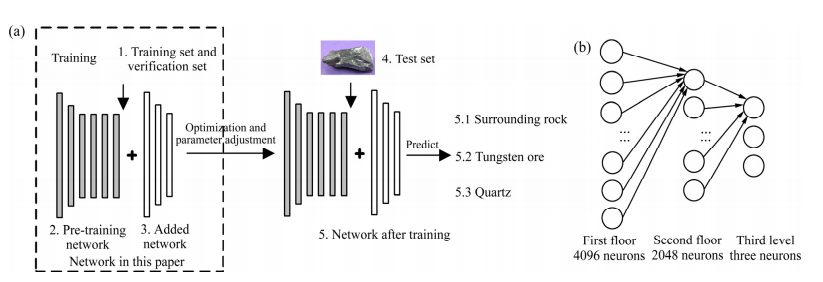
Fig. 3 Transfer learning method flow

Fig. 3 Transfer learning method flow: (a) Training flow; (b) Full connect layer neurons number

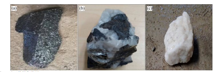
Fig. 4 Ore data set categories

Fig. 4 Ore data set categories: (a) Surrounding rock; (b) Tungsten ore; (c) Quartz

(3) Transfer Network Structure

This paper uses four improved Convolutional Neural Networks for transfer learning applied to the classification problem of tungsten ore, renaming the modified optimized networks as Wu-VGG19, Wu-V3, Wu-ResnetV2, and Wu-Resnet-50. Table 1 lists specific information about each network before modification. ImageNet is a database of images with manually labeled category tags (used for machine vision research), currently containing 22,000 categories. Since 2010, an ILSVRC software competition has been held annually based on this dataset, with software programs competing to classify and detect objects and scenes accurately. In the field of image classification, the accuracy in this competition has become a benchmark for computer vision classification algorithms. Since 2012, CNNs and deep learning have dominated the leaderboard in this competition, with the classification Test Top-5 accuracy now reduced to 2.25%.

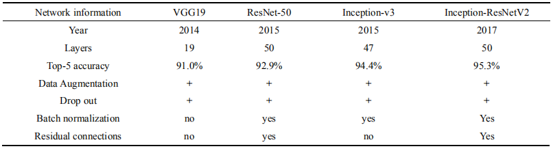
Table 1 Transfer network information

Table 1 Transfer network information

(4) Network Optimization and Environment Configuration

1) Network Optimization

The essence of network optimization is to minimize the loss function. All four networks in this paper adopt the Mini-batch gradient descent method to accelerate the model, balancing training speed and accuracy. The learning rate update strategy uses exponential decay. After testing, the learning rate for Wu-ResNetV2 is set to 0.001, while Wu-VGG19, Wu-V3, and Wu-Resnet-50 are set to 0.005, achieving good convergence effects for the transfer networks. The weight parameters (W) and bias parameters (b) of the added fully connected layers are randomly initialized in a certain manner, while the W and b of other layers are loaded from the weight file. The training epoch is set to 200, with cross-entropy used to calculate loss and a regularized loss function to mitigate overfitting.

2) Environment Configuration

The training and testing of the transfer network are based on the Keras framework, which is a high-level neural network API written in pure Python. Hardware environment: Intel(R) Core(TM) i7-7900X CPU @ 3.30GHz processor, 64GB memory, NVIDIA GeForce GTX 1080 Ti. GPU software environment: Ubuntu 16.04 64bit system, CUDA 5.0, CUDNN 8.0, Tensorflow-gpu-1.03, Keras 2.0, PyCharm professional version.

(1) Model Training and Testing Results

This paper’s training is mainly divided into two types: one is training to recognize two categories of tungsten ore and surrounding rock waste, addressing the issue of wolframite image recognition methods being unable to effectively distinguish between wolframite ore and surrounding rock waste; the other is training to recognize three categories: tungsten ore, black surrounding rock, and quartz, aimed at further distinguishing ores with significant grade differences to meet practical needs. Quartz is a gangue that generally contains smaller tungsten ore grains, and distinguishing ores of different grades has practical significance for improving beneficiation processes. This paper evaluates the training effect of a network based on indicators such as training accuracy (Train Accuracy), testing accuracy (Test Accuracy), and training loss (Loss). Training accuracy refers to the ratio of correctly output results by the model on the training set, calculated as follows:

(1)

In the formula: ntraincorrect indicates the number of correct identifications by the network in the training set; ntrainset indicates the number of samples in the training set. As the training dataset is relatively large, calculating the overall recognition accuracy for each training round would greatly extend the training time; therefore, only the training accuracy for each training batch is calculated, assuming each batch of samples meets the same distribution as the test set.

Testing accuracy refers to the ratio of correctly output results by the model on the test set, defined as follows:

(2)

This reflects the effectiveness of the network, which is a very important indicator. If the training accuracy and testing accuracy differ too much, it indicates that the network is overfitting, leading to poor generalization performance and impracticality. Therefore, a good network should aim to maximize testing accuracy while minimizing the gap between training and testing accuracy. The training process of the transfer network is essentially the process of minimizing the loss function, where Loss is the value of the loss function. The loss function essentially computes the mean squared error (MSE, Etrain) of the model on the test set, as shown in the formula:

(3)

1) Training Accuracy Comparison Analysis

The training results of the transfer networks for each group of experiments are shown in Figs. 5 and 6, where the training accuracy curves of the four transfer networks are depicted. The black line represents the training accuracy curve, and the gray line represents the validation accuracy curve; Fig. 7 shows the comparison of training accuracy (TrainAcc) curves and loss (Loss) curves for the four transfer networks.

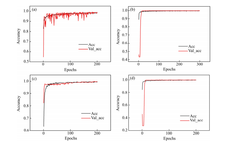
Fig. 5 TrainAcc diagram of two classification transfer networks

Fig. 5 TrainAcc diagram of two classification transfer networks: (a) 2-Wu-VGG19-TrainAcc; (b) 2-Wu-ResNet50-TrainAcc; (c) 2-Wu-V3-TrainAcc; (d) 2-Wu-ResNetV2-TrainAcc

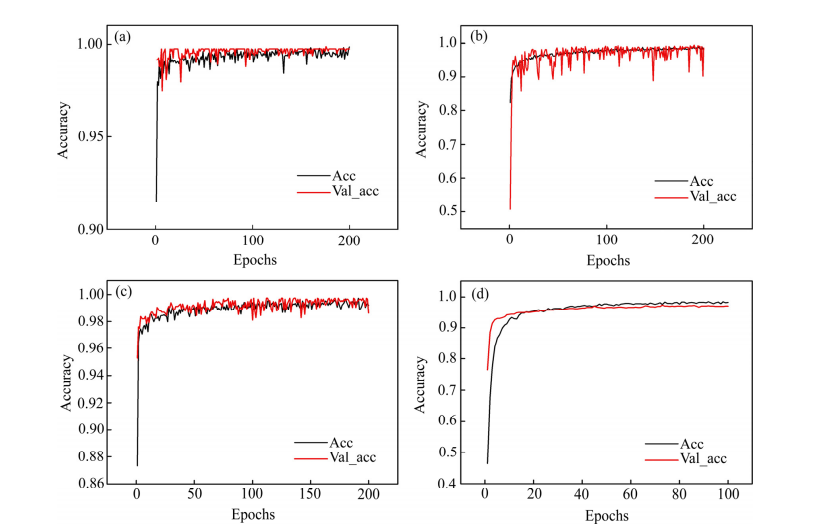
Fig. 6 TrainAcc diagram of three classification transfer networks

Fig. 6 TrainAcc diagram of three classification transfer networks: (a) 3-Wu-VGG19-TrainAcc; (b) 3-Wu-ResNet50-TrainAcc; (c) 3-Wu-V3-TrainAcc; (d) 3-Wu-ResNetV2-TrainAcc

From Fig. 5, after 200 training epochs, the final training accuracy for the four networks in the two-classification scenario exceeded 99%, with losses below 0.01. Wu-ResnetV2 achieved the best training data with a training accuracy of 99.89%, but Wu-VGG19 had the highest testing accuracy. From Fig. 6, similarly, in the three-classification scenario after 200 training epochs, the final training accuracy for the four networks exceeded 98%, with losses below 0.07; Wu-V3 achieved the best training data at 99.20%, but Wu-Resnet50 had the highest testing accuracy. These conclusions indicate that the best-performing network in testing among the four transfer networks selected in this paper is not necessarily the one with the best training results, as testing results are more meaningful in practice.

From Fig. 7, the four transfer networks in both two-class and three-class classifications converged rapidly within 10 epochs. This paper compared the testing accuracy of the three-class Wu-Resnet50 network trained for 50, 100, and 200 epochs, finding that as the training epochs increased, the testing accuracy of the transfer network gradually improved. Considering time costs and practical effects, this paper set the epoch to 200.

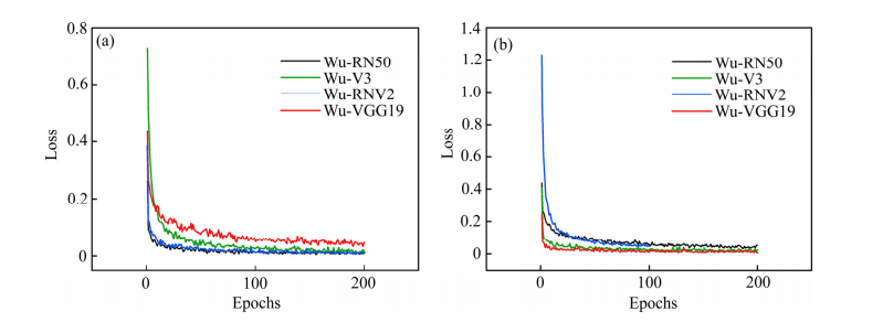
Fig. 7 Transfer networks training loss comparison diagram

Fig. 7 Transfer networks training loss comparison diagram: (a) Two-classification loss curve comparison; (b) Three-classification loss curve comparison

From Fig. 8, the difference between training accuracy and testing accuracy for the four transfer networks in two-class classification is significantly smaller than that in three-class classification, and the training accuracy is generally higher. In contrast, the testing accuracy of the same transfer network decreases for both two-class and three-class classifications. It can be seen that adding a new recognition category affects the performance of the transfer network, as the new category shares many similar features with the original categories, reducing the network’s recognition accuracy.

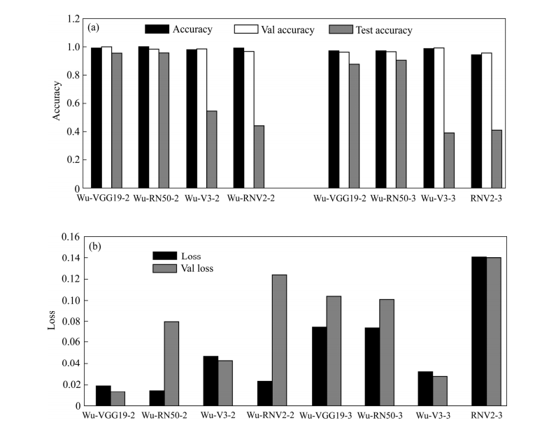
Fig. 8 Transfer networks accuracy and loss comparison diagrams

Fig. 8 Transfer networks accuracy and loss comparison diagrams: (a) Accuracy comparison; (b) Loss contrast

2) Testing Accuracy

The test images consist of images crawled from the internet and samples from other tungsten mines. The test set includes three categories of images: surrounding rock, tungsten ore, and quartz, equivalent to unknown samples. According to Table 2, in the two-class classification, Wu-VGG19 achieved the highest average testing accuracy of 95.85%, while in the three-class classification, Wu-Resnet50 achieved the highest average testing accuracy of 90.50%. The addition of a non-ore new category reduced the recognition accuracy of tungsten ore. In both two-class and three-class recognition tests, Wu-VGG19 and Wu-Resnet50 significantly outperformed other networks, indicating that different networks exhibit significant performance differences for different recognition tasks, necessitating a reasonable choice of recognition networks. Additionally, the Wu-VGG19 network, which performed best in the two-class classification, has the fewest layers, suggesting that merely deepening the network depth does not necessarily enhance recognition rates and may lead to overfitting.

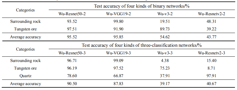
Table 2 Network test accuracy of two-classification and three-classification recognitions

Table 2 Network test accuracy of two-classification and three-classification recognitions

(2) Three-Class Optimization

The analysis results above indicate that Wu-v3 and Wu-ResNetv2 have testing classification accuracy significantly lower than the first two networks, and there are cases where one class has high classification accuracy while others are low. This may indicate overfitting or insufficient training, with fully connected layer parameters and insufficient datasets being significant causes of the above issues. Since this study only involves two or three classes, it may not require such complex fully connected layers, as this increases training difficulty. Therefore, the training strategies for Wu-v3 and Wu-ResNetv2 will be adjusted for further optimization.

Strategy One: Reduce the number of connection layers in the Wu-v3 and Wu-ResNetv2 networks (directly connect to the last layer) and retrain for three classifications. Strategy Two: Further augment the dataset to 2,500 images per category and retrain the Wu-v3 and Wu-ResNetv2 networks for three classifications, with testing accuracy shown in Table 3.

Comparing strategies one, two, and original training results, the Wu-ResNetv2 network adopted strategy one, resulting in a slight increase in average accuracy, but still exhibiting cases of one class having excessively high or low classification accuracy. Adopting strategy two improved average testing accuracy by 55.5%, with balanced testing accuracy across categories. The Wu-v3 network adopted strategy one, achieving a 57.77% increase in average testing accuracy, while strategy two led to a 55.63% increase in average testing accuracy, with balanced testing accuracy across categories. In summary, the Wu-ResNetv2 network’s recognition performance can be enhanced by augmenting the dataset, achieving an average accuracy of 96.17%. The Wu-v3 network can improve recognition accuracy by reducing fully connected layers or augmenting the dataset, achieving an average accuracy of 96.94%.

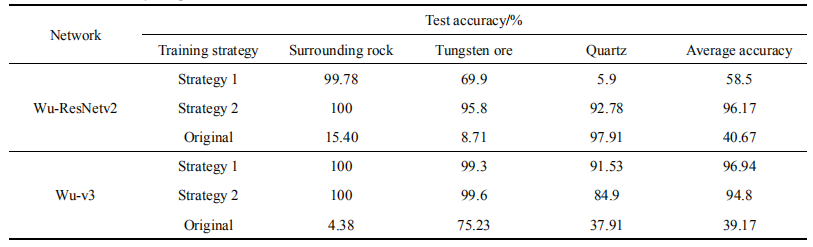
Table 3 Test accuracy of optimized three-classification network

Table 3 Test accuracy of optimized three-classification network

This paper believes that further research can be conducted in the following two areas:

1) In actual tungsten ore beneficiation, there are other categories of waste rock; adding new categories will significantly increase recognition difficulty, so further exploration of adding more categories for tungsten ore recognition is warranted;

2) Since the tungsten ore images captured on the manual selection belt consist of multiple ore blocks, achieving automated recognition of tungsten ore based on RGB images requires further research into target detection networks for recognizing multiple targets, in addition to hardware considerations.

2) The two improved transfer networks in this paper exhibit high recognition rates and good generalization performance, which is of significant practical importance for improving wolframite beneficiation processes. During the experiments, it was found that the best-performing network in testing among the four selected transfer networks is not necessarily the one with the best training results.

3) The Wu-VGG19 network, which has the optimal performance in two classifications, has the fewest layers, indicating that merely deepening the network depth does not necessarily enhance the recognition performance of tungsten ore. Issues of overfitting or insufficient training in three classifications can be resolved by reducing the fully connected layers or further augmenting the dataset.