Computer vision, natural language processing (NLP), and speech are the three main directions in deep learning research. Each of these fields has produced several classic modules used to model the different characteristics of the data they contain. The previous article introduced the design and core concepts of PaddleFluid and TensorFlow, and in this article, we start with image tasks, using PaddleFluid and TensorFlow to write an identical network, helping us understand how our usage experience can be transferred between different platforms, thus aiding our choice of convenient tools and focusing on the machine learning task itself.

In this article, we use SE_ResNeXt [1][2] as a practical task for image classification.

SE stands for Squeeze-and-Excitation, and the SE block is not a complete network structure but a substructure that can be embedded into other classification or detection models. The combination of SENet block and ResNeXt achieved first place in the ILSVRC 2017 classification project. It reduced the top-5 error rate on the ImageNet dataset from the previous best score of 2.991% to 2.251%.

How to Use the Code

This article comes with complete runnable code, including the following files:

Run the following command in the terminal to train the model using PaddleFluid. If no training data is detected in the cifar-10-batches-py directory under the current working directory (the cifar-10-batches-py folder does not need to be created manually), it will automatically download the training and test data from the network.

python SE_ResNeXt_fluid.py

Run the following command in the command line to train the model using TensorFlow, including model validation and model saving:

python SE_ResNeXt_tensorflow.py

Note:The latest code in this series can be found at TF2Fluid on GitHub [3].

Background Introduction

Convolutional neural networks have made significant breakthroughs in image-related tasks. Convolution kernels, as the core of convolutional neural networks, are typically viewed as aggregators of spatial information and channel information at the local receptive field. Typically, a convolution block consists of convolution layers, non-linear layers, and down-sampling layers (pooling layers), and a convolutional neural network is composed of a series of stacked convolution blocks. As the number of convolution blocks increases, the receptive field continues to expand, ultimately achieving the goal of capturing image features from a global receptive field for image description.

Squeeze-and-Excitation (SE) Module

Many research efforts in the image domain have explored how to construct more powerful networks to learn image features from different perspectives. For example, the Inception structure embeds multi-scale information: using multiple convolution kernels of different sizes to aggregate features from various receptive fields for performance gains; introducing attention mechanisms into the spatial dimensions, etc., have all achieved considerable success.

Besides these angles, it is natural to consider whether we can enhance network performance by considering the relationships between feature channels. This is precisely the design motivation of the Squeeze-and-Excitation module.

The SE block consists of two critical operations, Squeeze and Excitation, with the core idea being to explicitly model the interdependencies between feature channels, adaptively learning the importance of each feature channel, and then enhancing useful features (increasing the weight of useful feature maps) while suppressing features that are not useful for the current task (decreasing the weight of ineffective or minimally effective feature maps), achieving better model performance.

The following figure illustrates the SE Block, sourced from reference [1] Figure 1.

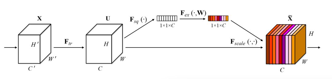
▲ Figure 1. SE Block Illustration

Squeeze Operation, in Figure 1:

Through a global pooling operation, features are compressed along the spatial dimension, transforming each two-dimensional feature channel into a real number. This real number has a certain degree of global receptive field. The output dimension of the Squeeze operation is equal to the number of feature channels in the input feature map, representing the global distribution of responses along the feature channel dimension. Squeeze allows layers closer to the input to gain a global receptive field, which is very useful in many tasks.

Excitation Operation, in Figure 1:

Similar to a gating mechanism. By applying the parameter WW, a weight is learned for each feature channel, where the learnable parameter WW is used to explicitly model the correlations between feature channels.

Scale Weighting Operation:

The final step treats the weights output from Excitation as the importance of each feature channel after feature selection, and then reweights the original features channel-wise through scaling, completing the recalibration of the original features along the channel dimension.

When the SE block is embedded into existing classification networks, it inevitably increases the number of parameters to be learned and introduces computational overhead. However, the computational cost brought by the SE block is relatively low, and the improvement in performance remains substantial, making it acceptable for most tasks.

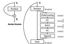
SE Module and Residual Connection Overlay

Figure 2 illustrates the principle of overlaying the SE module with the Residual Connection in ResNet, sourced from reference [1] Figure 3.

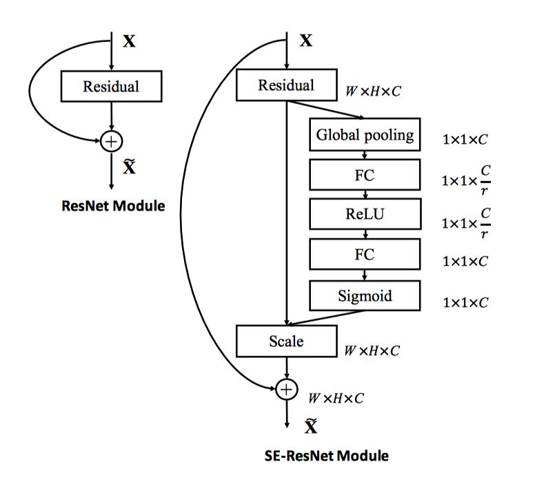
▲ Figure 2. SE Module and Residual Connection Overlay

The SE module can be embedded into models that contain Residual Connections in ResNet. The right side of Figure 2 shows the illustration of SE overlaying the Residual Connection. The paper suggests overlaying the SE module before the Addition operation in the cross-layer connection of the Residual Connection, rather than after the Addition operation: this is because the features of the Residual on the branch have undergone feature recalibration, and if there exists a scale operation (extraction step) on the backbone with a range of 0 to 1, it is easy for the gradient to vanish when the backpropagation algorithm reaches the layers close to the input in deeper networks, making it difficult to optimize the model.

ResNeXt Model Structure

To improve the accuracy of deep learning methods, one typically chooses to deepen or widen the network. However, as the depth or width of the network increases, the number of parameters (e.g., feature channel count, filter size, etc.) also significantly increases, raising computational overhead. The design intention of the ResNeXt network structure is to improve network performance without increasing parameter complexity while also reducing the number of hyperparameters.

Before introducing the ResNeXt network, we first review two very important works in the field of image classification: VGG and Inception networks (the design details of these two networks are described in detail in the image classification section of PaddleBook [4] ).

The VGG network constructs deep networks by stacking the same-shaped network modules, a simple strategy that was similarly employed by ResNet later. This strategy reduces the complexity of hyperparameter selection and works effectively across many different datasets and tasks, demonstrating good robustness.

The Inception network’s result is carefully designed, following the split-transform-merge strategy. In an Inception model: (1) split: the input is split into several low-dimensional feature maps using a 1×1 convolution; (2) transform: the output of the split step is transformed through a set of (multiple) filters of different sizes; (3) merge: the results from the transform step are merged through concatenation.

The Inception model aims to approximate the expressive power of large dense filters with a lower computational cost. Although the Inception model achieves good accuracy, each Inception module requires customization of the number and size of filters, and the module must change at each stage, especially when adapting the Inception module to new data or tasks, which lacks a particularly universal method.

ResNeXt combines the advantages of VGG and Inception, proposing a simple architecture: adopting the strategy of repeating the same network layer from VGG/ResNets in a straightforward and scalable way, continuing the split-transform-merge strategy, where all building blocks of the network are the same, and there is no need to adjust the hyperparameters of each building block at every stage; simply stacking identical building blocks can form the entire network.

Figure 3, sourced from reference [2] Figure 1, illustrates the basic building block of the ResNeXt network.

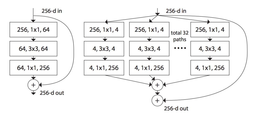
▲ Figure 3. Basic Building Block of ResNeXt Network

Before explaining Figure 3, we need to introduce a term: cardinality, which refers to the size of the set of transformations in the building block. In Figure 3, cardinality=32, meaning that the 64 convolution kernels on the left are divided into 32 different paths on the right, and the output vectors from the 32 paths are summed at corresponding positions, and then added to the Residual connection.

Combining Figure 3 with the previous section’s discussion of “SE Module and Residual Connection Overlay” forms the final building block of the SE_ResNeXt network, which can be stacked to create the entire ResNeXt.

CIFAR-10 Dataset Introduction

Having introduced the principles and basic structure of the ResNeXt model, we are ready to start building training tasks using PaddleFluid and TensorFlow.

In this article, we use the cifar10 dataset [5][6] as experimental data. The cifar-10 dataset contains 60,000 32*32 color images, divided into 10 categories. Figure 4 illustrates the 10 categories of the cifar-10 dataset.

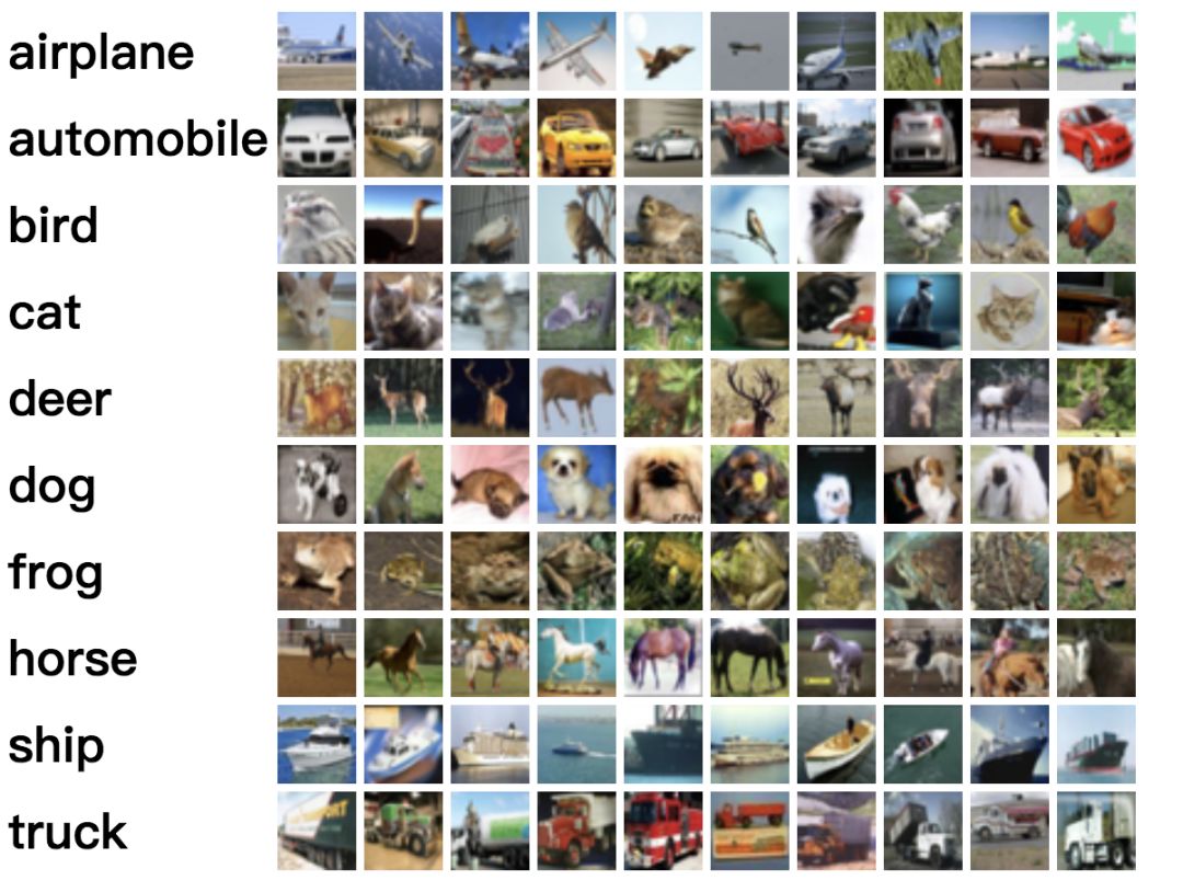
▲ Figure 4. CIFAR-10 Dataset

The cifar10 dataset contains 50,000 training images and 10,000 test images, divided into 5 training batches and 1 test batch, with each batch containing 10,000 images. The test batch contains 1,000 images randomly selected from each category.

Download Data

When running the training program, if there is no cifar-10-batches-py directory in the current execution directory, or if there is no pre-downloaded data in the cifar-10-batches-py directory, the data reading modules of PaddleFluid and TensorFlow will automatically call the download_data method in data_utils [7] to download the cifar-10 dataset from the website without manual downloading.

Loading CIFAR-10 Dataset

PaddleFluid

1. Define the input layer of the network:

In the previous basic usage concept, PaddleFluid models receive input data through fluid.layers.data. The image classification network takes images and their corresponding category labels as input:

IMG_SHAPE = [3, 32, 32]

images = fluid.layers.data(name="image", shape=IMG_SHAPE, dtype="float32")
labels = fluid.layers.data(name="label", shape=[1], dtype="int64")

In the above code snippet, the shape specified in fluid.layers.data does not require explicitly specifying the 0th dimension batch size; the framework will automatically supplement the 0th dimension and fill the correct batch size during runtime.

An image is a 3-D Tensor. PaddleFluid uses a channel-first data input format for convolution operations. Therefore, when receiving raw image data, the three dimensions of the shape represent: channel, image width, and image height.

2. Using a data reader function written in Python

PaddleFluid uses the DataFeeder interface to feed data to fluid.data.layersfeed, called as follows:

train_reader = paddle.batch(train_data(), batch_size=conf.batch_size)
feeder = fluid.DataFeeder(place=place, feed_list=[images, labels])

In the above code snippet:

1. Users only need to write the train_data() Python generator. This function is the data reader interface required by PaddleFluid, and the function name is not limited.

2. When implementing this data reader interface, one only needs to consider: how to read data from the raw data file and return a single training data point in numpy ndarray format.

3. Calling paddle.batch(train_data(), batch_size=conf.batch_size) will first read the data into a pool, shuffle it, and then sequentially take one mini-batch from the pool.

For the complete code, please refer to train_data() [8], and it will not be pasted directly here.

TensorFlow

1. Define a placeholder

In TensorFlow, a special tensor called a placeholder is defined to accept input data.

IMG_SHAPE = [3, 32, 32]
LBL_COUNT = 10

images = tf.placeholder(
    tf.float32, shape=[None, IMG_SHAPE[1], IMG_SHAPE[2], IMG_SHAPE[0]])
labels = tf.placeholder(tf.float32, shape=[None, LBL_COUNT])

It is important to note that:

TensorFlow’s convolution operations default to using a channel-last data format (it can also use a channel-first data format when calling convolution interfaces), and the shape of this placeholder differs from the shape of images in PaddleFluid.

In the placeholder, the dimension for the batch size can be determined at runtime, using None as a placeholder.

2. Providing data for placeholders via a feeding dictionary

TensorFlow manages the execution of a computation graph through sessions. When calling the session’s run method, a feeding dictionary is provided to feed mini-batch data to the placeholder.

The following code snippet implements loading cifar-10 data for training.

image_train, label_train = train_data()
image_test, label_test = train_data()
total_train_sample = len(image_train)

for epoch in range(1, conf.total_epochs + 1):
        for batch_id, start_index in enumerate(
                range(0, total_train_sample, conf.batch_size)):
            end_index = min(start_index + conf.batch_size,
                            total_train_sample)
            batch_image = image_train[start_index:end_index]
            batch_label = label_train[start_index:end_index]

            train_feed_dict = {
                images: batch_image,
                labels: batch_label,
               ......
            }

The train_data() function in the above code snippet [7] completes the reading of the raw data. Unlike PaddleFluid, where only reading a single data point is required and the framework handles batching, in TensorFlow, train_data reads all data, with user programs controlling shuffling and batching.

Constructing the Network Structure

The core of using different deep learning frameworks is constructing neural network model structures using the operators provided by the frameworks. Detailed descriptions of the basic operators provided by PaddleFluid and TensorFlow can be found on their respective official websites.

This article provides the code files SE_ResNeXt_fluid.py [9] and SE_ResNeXt_tensorflow.py [10], which are the ResNeXt networks written in PaddleFluid and TensorFlow, respectively. The network structures in both files are completely identical, and the code structure is also entirely the same. The core is the SE_ResNeXt class, as shown in the following code snippet:

class SE_ResNeXt(object):
    def __init__(self, x, num_block, depth, out_dims, cardinality,
                 reduction_ratio, is_training):
        ...

    def transform_layer(self, x, stride, depth):
        ...

    def split_layer(self, input_x, stride, depth, layer_name, cardinality):
        ...

    def transition_layer(self, x, out_dim):
        ...

    def squeeze_excitation_layer(self, input_x, out_dim, reduction_ratio):
        ...

    def residual_layer(self, input_x, out_dim, layer_num, cardinality, depth,
                       reduction_ratio, num_block):
        ...

    def build_SEnet(self, input_x):
        ...

The SE_ResNeXt_fluid.py [9] and SE_ResNeXt_tensorflow.py [10] files contain the same member functions in the SE_ResNeXt class, allowing for comparison to understand how to transfer usage experience between the two platforms by implementing the same functionality in both.

Differences in 2-D Convolution Layers

2-D convolution is a crucial operation in image tasks, where the convolution kernel shifts across two axes, multiplying each element of the convolution kernel with the corresponding position in the convolved image and summing the results. The continuous movement of the convolution kernel outputs a new image, composed entirely of the summed products of the convolution kernel at various positions. Figure 5 visualizes the computation process of 2-D convolution when the input image is a 4-D Tensor (with the batch size fixed at 1, meaning the first dimension of the 4-D Tensor is fixed at 1).

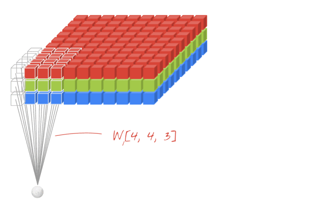
▲ Figure 5. 2-D Convolution on RGB 3-Channel Image Input

Author: Martin Görner / Twitter: @martin_gorner

Some details of convolution computation differ slightly between PaddleFluid and TensorFlow, which we will explain here.

Below is the PaddleFluid 2-D convolution calling interface:

fluid.layers.conv2d(
  input,
  num_filters,
  filter_size,
  stride=1,
  padding=0,
  dilation=1,
  groups=None,
  act=None,
  ...)

1. PaddleFluid uses a “channel-first” data input format for convolution, commonly referred to as the “NCHW” format.

If the input image is in a “channel-last” format, the fluid.layers.transpose operator can be added before the convolution operation to reorder the axes of the input data.

2. In PaddleFluid, users need to calculate the padding property for convolution computations. The height and width of the output image are calculated using the following formula:

The padding property can accept a Python list with two elements, specifying padding for the height and width directions of the image. If padding is an integer rather than a list, it is assumed that the height and width padding are the same number of zeros.

This logic also applies to the stride and dilation parameters.

Below is the TensorFlow 2-D convolution calling interface:

tf.layers.conv2d(
  inputs,
  filters,
  kernel_size,
  strides=(1, 1),
  padding='valid',
  data_format='channels_last'
  ...)

1. TensorFlow’s convolution defaults to using a “channel-last” data input format, commonly referred to as the “NHWC” format.

2. In TensorFlow, the padding property for convolution can specify two modes: “valid”: no padding; “same”: the output image’s width and height after convolution will be the same as the input image.

Differences in Regularization Terms

L2 regularization is one of the means to prevent overfitting and plays an important role in the training of neural networks. The interfaces for adding L2 regularization differ slightly between the PaddleFluid and TensorFlow platforms.

PaddleFluid

In PaddleFluid, using L2 regularization as a standard regularization term is relatively simple; L2 regularization is a parameter of the optimizer, and the regularization coefficient is passed directly.

optimizer = fluid.optimizer.Momentum(
    learning_rate=conf.learning_rate,
    momentum=0.9,
    regularization=fluid.regularizer.L2Decay(conf.weight_decay))

TensorFlow

In TensorFlow, L2 regularization is part of the loss function, requiring explicit addition of L2 regularization for each learnable parameter that needs it.

l2_loss = tf.add_n([tf.nn.l2_loss(var) for var in tf.trainable_variables()])

optimizer = tf.train.MomentumOptimizer(
    learning_rate=learning_rate,
    momentum=conf.momentum,
    use_nesterov=conf.use_nesterov)
train = optimizer.minimize(cost + l2_loss * conf.weight_decay)

The above sections highlight some differences to pay attention to when using PaddleFluid and TensorFlow. Other interface calling details for training the ResNeXt model on both platforms can be found in the code of SE_ResNeXt_fluid.py and SE_ResNeXt_tensorflow.py, and we will not paste all the code here. The entire process follows:

• Define the network structure;

• Load training data;

• In a for loop, read mini-batch data one by one, call the network’s forward and backward computations, and invoke the optimization process.

Summary

In this article, we approached the image classification problem in the image domain, using PaddleFluid and TensorFlow to implement the identical ResNeXt network structure to introduce:

1. How to read and feed image data to the network in PaddleFluid and TensorFlow;

2. How to use 2-D convolution, 2-D pooling, padding, and other commonly used computational units in image tasks in PaddleFluid and TensorFlow;

3. How to run a complete training task, testing samples from the test set during training.

It can be seen that the image operation interfaces of PaddleFluid and TensorFlow are highly similar. PaddleFluid supports a rich set of image operations similar to TensorFlow, which is a common choice among today’s mainstream deep learning frameworks. As users, our usage experience can be easily transferred between platforms, requiring only slight attention to differences in interface calling details.

In the upcoming chapters, we will further compare how to use recurrent neural network units in PaddleFluid and TensorFlow to handle sequential input data in NLP tasks, and gradually introduce topics such as multi-threading and multi-card training.

References

[1]. Hu J, Shen L, Sun G. Squeeze-and-excitation networks[J]. arXiv preprint arXiv:1709.01507, 2017.

[2]. Xie S, Girshick R, Dollár P, et al. Aggregated residual transformations for deep neural networks[C]//Computer Vision and Pattern Recognition (CVPR), 2017 IEEE Conference on. IEEE, 2017: 5987-5995.

[3]. TF2Fluid: https://github.com/JohnRabbbit/TF2Fluid

[4]. PaddleBook Image Classification

http://www.paddlepaddle.org/docs/develop/book/03.image_classification/index.cn.html

[5]. Learning Multiple Layers of Features from Tiny Images, Alex Krizhevsky, 2009.

https://www.cs.toronto.edu/~kriz/learning-features-2009-TR.pdf

[6]. The CIFAR-10 dataset: https://www.cs.toronto.edu/~kriz/cifar.html

[7]. data_utils

https://github.com/JohnRabbbit/TF2Fluid/blob/master/02_image_classification/data_utils.py#L35

[8]. train_data()

https://github.com/JohnRabbbit/TF2Fluid/blob/master/02_image_classification/cifar10_fluid.py#L43

[9]. SE_ResNeXt_fluid.py

https://github.com/JohnRabbbit/TF2Fluid/blob/master/02_image_classification/SE_ResNeXt_fluid.py

[10]. SE_ResNeXt_tensorflow.py

https://github.com/JohnRabbbit/TF2Fluid/blob/master/02_image_classification/SE_ResNeXt_tensorflow.py

#Welfare Time#

Here comes the simple and straightforward welfare session

PaperWeekly × PaddlePaddle

Deep Learning Survey with Prizes

50 prizes waiting to be claimed

Limited Edition T-Shirts√ Whiteboards√ Mechanical Keyboards√

How to Participate

Scan the QR code below to submit the questionnaire

▼

We will randomly select 50 users who successfully answer to receive a limited edition gift 🎁