Illustration Of Transformer Architecture

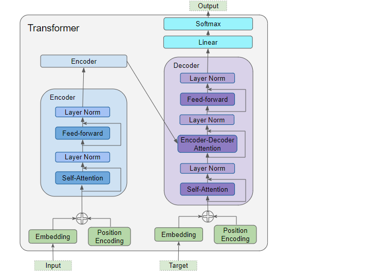
1. Overview

The overall architecture of the Transformer has been introduced in the first section:

1. Data must go through the following before entering the encoder and decoder:

• Embedding Layer

• Positional Encoding Layer

1. The encoder stack consists of several encoders. Each encoder contains:

• Multi-Head Attention Layer

• Feed Forward Layer

1. The decoder stack consists of several decoders. Each decoder contains:

• Two Multi-Head Attention Layers

• Feed Forward Layer

1. The output produces the final output:

• Linear Layer

• Softmax Layer.

To deeply understand the role of each component, we will train the Transformer step-by-step in a translation task using a training dataset with only one sample, which includes an input sequence (“You are welcome” in English) and a target sequence (“De nada” in Spanish).

2. Embedding Layer and Positional Encoding

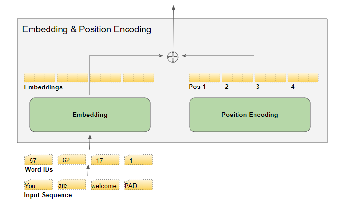
The input to the Transformer needs to focus on two pieces of information for each word: the meaning of the word and its position in the sequence.

1. The first piece of information can be encoded through the embedding layer to represent the meaning of the word.

2. The second piece of information can be represented by the positional encoding layer to indicate the position of the word.

The Transformer accomplishes the encoding of these two different pieces of information by adding two layers.

1. Embedding Layer

Each of the encoder and decoder in the Transformer has an embedding layer.

In the encoder, the input sequence is fed into the embedding layer of the encoder, referred to as Input Embedding.

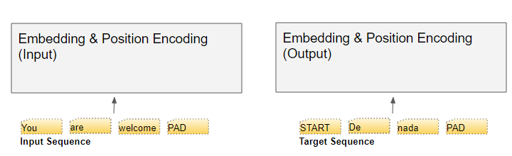
In the decoder, the target sequence is shifted one position to the right, and a Start token is inserted at the first position before being fed into the embedding layer of the decoder. Note that during inference, we do not have the target sequence, but instead, we cyclically feed the output sequence into the embedding layer of the decoder, as mentioned in the first article. This process is referred to as Output Embedding.

Each text sequence is mapped to a sequence of word IDs in the vocabulary before entering the input embedding layer. The embedding layer then projects each numerical sequence into an embedding vector, which provides a richer representation of the meaning of the word.

2. Positional Encoding

In RNNs, each word is input in sequence, inherently knowing the position of each word.

However, in the Transformer, all words in a sequence are input in parallel. This is a major advantage over RNN architectures; however, it also means that positional information is lost and needs to be added back separately.

Both the decoder stack and the encoder stack have a positional encoding layer. The computation of positional encoding is independent of the input sequence, is a fixed value, and only depends on the maximum length of the sequence.

1. The first term is a constant code representing the first position.

2. The second term is a constant code representing the second position.

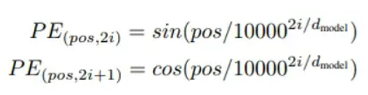
pos is the position of the word in the sequence, d_model is the length of the encoding vector (which is the same as the embedding vector), and i is the index of this vector. The formula represents the elements at the pos row and the 2i and (2i+1) columns of the matrix.

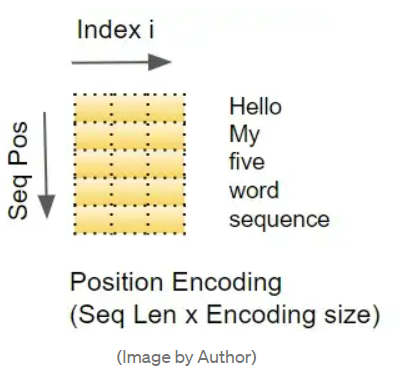
In other words, positional encoding interweaves a series of sine curves and a series of cosine curves. For each position pos, when i is even, the sine function is used for calculation; when i is odd, the cosine function is used for calculation.

3. Matrix Dimensions

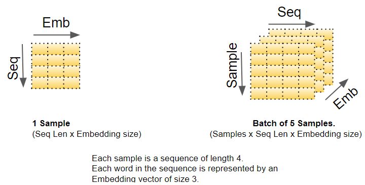
Deep learning models process a batch of training samples at a time. The embedding layer and positional encoding layer operate on a matrix of a batch of sequence samples. The embedding layer accepts a 2D word ID matrix of shape (samples, sequence_length) and encodes each word ID into a word vector of size embedding_size, resulting in a 3D output matrix of shape (samples, sequence_length, embedding_size). The encoding size used by the positional encoding is equal to the embedding size. Thus, it produces a similarly shaped matrix that can be added to the embedding matrix.

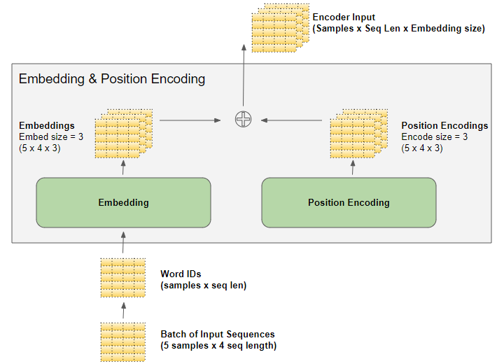
The (samples, sequence_length, embedding_size) shape produced by the embedding layer and positional encoding layer is preserved in the model, flowing with the data through the encoder and decoder stacks until it is altered by the final output layer. [It actually becomes (samples, sequence_length, vocab_size)].

The above provides an intuitive understanding of the matrix dimensions in the Transformer. To simplify visualization, from here on, we will temporarily drop the first dimension (samples dimension) and use a 2D representation of a single sample.

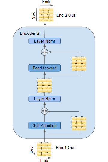
4. Encoder

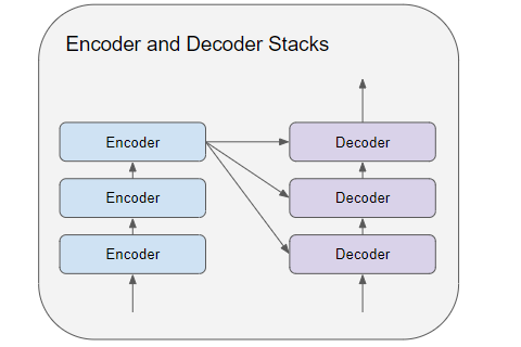
The encoder and decoder stacks each consist of several (usually 6) encoders and decoders connected in sequence.

1. The first encoder in the stack receives its input from the embedding and positional encoding. The other encoders in the stack receive their input from the previous encoder.

2. The current encoder accepts the input from the previous encoder and passes it to the self-attention layer of the current encoder. The output of the current self-attention layer is passed to the feed forward layer and then output to the next encoder.

1. Both the self-attention layer and the feed-forward network have a residual connection and are then sent to a normalization layer. Note that there is also a residual connection when the input from the previous decoder enters the current decoder.

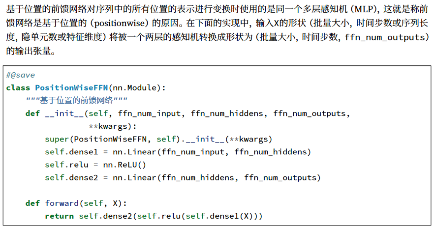
2. Reference: In the book by Professor Li Mu, “Deep Learning with Hands-On Practice”, page 416 has a detailed explanation of the “Position-based Feed Forward Network”. Specifically, this feed-forward network consists of a linear layer, an activation function, and another linear layer. Moreover, this feed-forward network does not change the shape of the input.

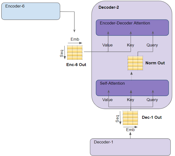
The output of the last encoder in the encoder stack is fed into each decoder in the decoder stack.

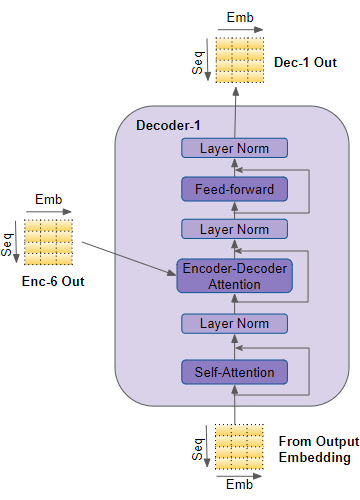
5. Decoder

The structure of the decoder is very similar to that of the encoder, but with some differences.

1. Like the encoder, the first decoder in the decoder stack receives input from the embedding layer (word embedding + positional encoding); the other decoders in the stack receive input from the previous decoder.

2. Within a decoder, the input first goes into the self-attention layer, which operates differently from the self-attention layer in the encoder:

• During training, the self-attention layer of the decoder receives the entire output sequence. However, to avoid seeing future data (i.e., to prevent information leakage) when generating each output, a technique called “masking” is used, ensuring that when generating the i-th word, the model can only see the first word to the i-th word.

• During inference, the input at each time step is the entire output sequence generated up to the current time step.

1. Another difference between the decoder and encoder is that the decoder has a second attention layer, namely the Encoder-Decoder Attention Layer. Its operation is similar to the self-attention layer, except that its input comes from two places: the output of the self-attention layer and the output of the decoder stack.

2. The output of the Encoder-Decoder Attention layer is passed to the feed-forward layer and then to the next decoder.

3. Each sub-layer in the decoder, including the self-attention layer, encoder-decoder attention layer, and feed-forward layer, has a residual connection and undergoes layer normalization.

6. Attention

In the first part, we discussed why the attention mechanism is so important. In the Transformer, attention is used in three places:

1. Self-attention in the Encoder: Attention computation of the input sequence on itself;

2. Self-attention in the Decoder: Attention computation of the target sequence on itself;

3. Encoder-Decoder Attention in the Decoder: Attention computation of the target sequence on the input sequence.

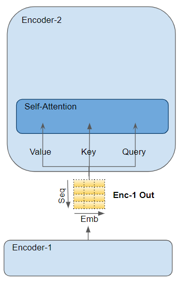
The attention layer is computed using three parameters known as Query, Key, and Value:

1. In the self-attention of the Encoder, the input of the encoder is multiplied by the corresponding parameter matrices to obtain Query, Key, and Value.

1. In the self-attention of the Decoder, the input of the decoder obtains Query, Key, and Value in the same way.

2. In the Encoder-Decoder attention of the decoder, the output of the last encoder in the encoder stack is passed to the Value and Key parameters. The output of the self-attention and Layer Norm modules from the Encoder-Decoder attention is passed to the Query parameter.

7. Multi-Head Attention

The Transformer refers to each attention calculation unit as an Attention Head. Multiple attention heads perform parallel computations, which is known as Multi-head Attention. This enhances the attention computation’s ability to resolve by integrating several identical attention calculations.

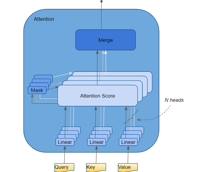
Each independent linear layer has its own weight parameters, namely Query, Key, and Value, which are multiplied with the input to obtain Q, K, and V. These results are combined using the attention formula shown below to produce the Attention Score.

It is important to note that the values of Q, K, and V are the encoded representations of each word in the sequence. The attention computation connects each word with other words in the sequence, encoding an Attention Score for each word in the sequence.

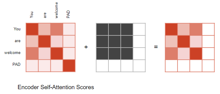
8. Attention Masks

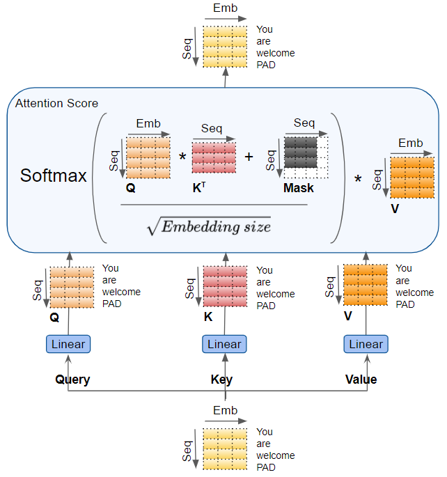
While calculating the Attention Score, the Attention module applies a masking operation. The masking operation serves two purposes:

1. In the Self-attention and Encoder-Decoder attention of the Encoder: The role of the mask is to zero out the output attention scores at the positions corresponding to padding in the input sequence, ensuring that padding does not contribute to the Self-attention computation.

• The role of padding: Since input sequences may have different lengths, padding is used as a filler token, similar to most NLP methods, to obtain fixed-length vectors, allowing a sequence of one sample to be input into the Transformer as a matrix.

• When calculating the Attention Score, the masking is applied to the numerator before the Softmax computation. The masked elements (white squares) are set to negative infinity, so that Softmax turns these values into zero.

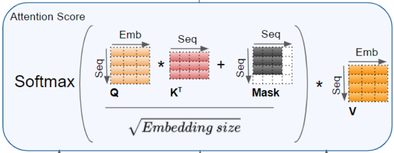
Illustration of the padding mask operation:

The masking operation in the Encoder-Decoder attention is similar:

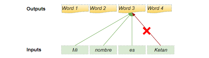
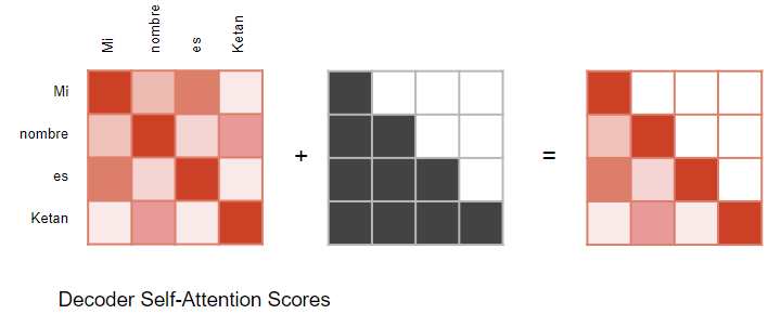
1. In the Self-attention of the Decoder: The masking serves to prevent the decoder from “sneaking a peek” at the remaining parts of the target sentence during prediction at the current time step:

• The decoder processes the words in the source sequence and uses them to predict the words in the target sequence. During training, this process is done using Teacher Forcing, where the complete target sequence is used as input to the decoder. Therefore, when predicting a particular position’s word, the decoder can use both the previous target words and the later target words. This allows the decoder to “cheat” by using target words from future “time steps”.

• For example, as shown in the figure below, when predicting “Word3”, the decoder should only reference the first three input words of the target words, excluding the fourth word “Ketan”. Thus, the Self-attention mask operation in the Decoder masks the target words located after the current time step in the sequence.

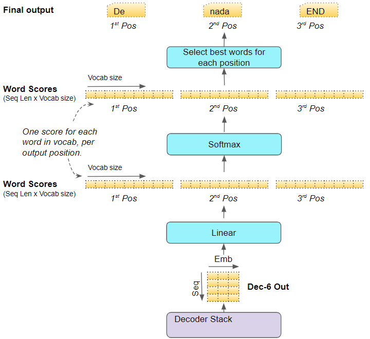
9. Generate Output

The last decoder in the decoder stack passes its output to the output component, which converts it into the final target sentence.

1. The linear layer projects the decoder vector to word scores, where each unique word in the target vocabulary has a score value at each position in the sentence. For example, if our final output sentence has 7 words and the target Spanish vocabulary has 10,000 unique words, we generate 10,000 score values for each of these 7 words. The score values indicate the likelihood of each word in the vocabulary appearing at that position in the sentence.

2. The Softmax layer converts these scores into probabilities (summing to 1.0). At each position, we find the index of the word with the highest probability (greedy search) and map that index to the corresponding word in the vocabulary. These words form the output sequence of the Transformer.

10. Training and Loss Function

During training, cross-entropy is used as the loss function to compare the generated output probability distribution with the target sequence. The probability distribution gives the probability of each word appearing at that position.

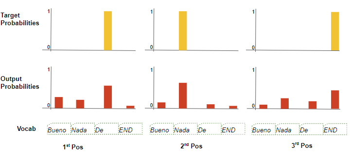
Assuming our target vocabulary contains only four words. Our goal is to produce a probability distribution that matches our expected target sequence “De nada END”.

This means that in the probability distribution for the first word position, the probability of “De” should be 1, while the probabilities of all other words in the vocabulary should be 0. Similarly, in the second and third word positions, the probabilities of “nada” and “END” should both be 1, while the probabilities of other words in the vocabulary should be 0.

As usual, the loss is computed, and gradients are calculated to train the model through backpropagation.